
library(vernissage)
labs <- c(AGE = "Age (years)", BMI = "BMI", SEX = "Sex", NFL_V0 = "NfL V0", IL6_V0 = "IL-6 V0",
          CRP_V0 = "CRP V0", MOCA_V0 = "MoCA V0", UPDRS_V0 = "UPDRS-III V0", FALL_V0 = "Falls V0",
          GROUP = "Arm")
The cohort overview table
describe_cohort() is the first table of an analysis: type, number observed, missing values, summaries overall and by group, a group comparison and a small histogram of each variable.
describe_cohort(cohort_sim,
                vars = c(AGE, SEX, BMI, NFL_V0, IL6_V0, CRP_V0, MOCA_V0, UPDRS_V0, FALL_V0),
                by = GROUP, id_col = ID, labels = labs,
                blocks = list(Demography = c("AGE", "SEX", "BMI"),
                              Biomarkers = c("NFL_V0", "IL6_V0", "CRP_V0"),
Clinical = c("MOCA_V0", "UPDRS_V0", "FALL_V0")))| Cohort overview | |||||||||
| 120 subjects (120 unique identifiers) | 9 variables | 111 complete subjects (92%) | by Arm | |||||||||
| Variable | Type | N | Missing | Overall (n = 120) |
Range |
Arm
|
p | Distribution | |
|---|---|---|---|---|---|---|---|---|---|
| Placebo (n = 67) |
Active (n = 53) |
||||||||
| Demography | |||||||||
| Age (years) | Continuous | 120 | 0 (0%) | 67.0 [61.0; 71.0] | 45.0 to 86.0 | 68.0 [61.0; 71.0] | 66.0 [62.0; 70.0] | 0.55 | ▁▁▅▆█▅▂▂ |
| Sex | Binary | 120 | 0 (0%) | 0.64 | |||||
| Female | 47 (39%) | 28 (42%) | 19 (36%) | ████ | |||||
| Male | 73 (61%) | 39 (58%) | 34 (64%) | ██████ | |||||
| BMI | Continuous | 116 | 4 (3%) | 26.0 [23.5; 28.6] | 16.7 to 33.1 | 26.0 [23.4; 28.8] | 26.1 [23.6; 28.4] | 0.88 | ▂▂▄▇██▅▄ |
| Biomarkers | |||||||||
| NfL V0 | Continuous | 120 | 0 (0%) | 13.0 [8.4; 17.3] | 4.1 to 69.4 | 13.0 [8.1; 17.6] | 13.2 [9.0; 17.2] | 0.92 | █▇▂▁▁ ▁ |
| IL-6 V0 | Continuous | 120 | 0 (0%) | 1.1 [0.7; 1.7] | 0.5 to 7.8 | 1.0 [0.7; 1.5] | 1.3 [0.7; 2.1] | 0.17 | █▃▁▁▁▁ ▁ |
| CRP V0 | Continuous | 115 | 5 (4%) | 1.9 [1.2; 3.4] | 0.1 to 31.3 | 2.0 [1.3; 3.8] | 1.8 [1.0; 3.1] | 0.27 | █▂▁▁▁ ▁ |
| Clinical | |||||||||
| MoCA V0 | Discrete | 120 | 0 (0%) | 27.0 [25.8; 29.0] | 21.0 to 30.0 | 27.0 [25.5; 28.0] | 27.0 [26.0; 29.0] | 0.75 | ▁▂▂▄▆▄▅█ |
| UPDRS-III V0 | Continuous | 120 | 0 (0%) | 24.0 [18.0; 31.0] | 1.0 to 46.0 | 22.0 [18.0; 31.0] | 25.0 [17.0; 31.0] | 0.69 | ▂▄▄███▄▁ |
| Falls V0 | Binary | 120 | 0 (0%) | 1 | |||||
| No | 96 (80%) | 54 (81%) | 42 (79%) | ████████ | |||||
| Yes | 24 (20%) | 13 (19%) | 11 (21%) | ██ | |||||
| Continuous / discrete: median [Q1; Q3] and range; categorical: n (%) of the observed values. Missing: n (% of subjects). Distribution: histogram of the observed values (8 bins) or share of each level. p: Wilcoxon / Chi², unadjusted (description only). | |||||||||
The same content is available as a tibble with output = "data".
Missing data
na_summary(cohort_sim, list(Biomarkers = c("NFL_V0", "NFL_V3", "IL6_V3", "CRP_V0"),
                            Scores = c("MOCA_V3", "UPDRS_V3")))
#> # A tibble: 6 × 5
#>   Block      Variable Label    N_missing Pct_missing
#>   <chr>      <chr>    <chr>        <int>       <dbl>
#> 1 Scores     MOCA_V3  MOCA_V3         14        11.7
#> 2 Biomarkers NFL_V3   NFL_V3          13        10.8
#> 3 Biomarkers IL6_V3   IL6_V3          10         8.3
#> 4 Scores     UPDRS_V3 UPDRS_V3        10         8.3
#> 5 Biomarkers CRP_V0   CRP_V0           5         4.2
#> 6 Biomarkers NFL_V0   NFL_V0           0         0
na_complete_cases(cohort_sim, list(Baseline = c("NFL_V0", "IL6_V0", "CRP_V0", "MOCA_V0"),
                                   `Both visits` = c("NFL_V0", "NFL_V3", "MOCA_V0", "MOCA_V3")))
#> # A tibble: 2 × 4
#>   `Variable set` `N variables` `N complete` `% complete`
#>   <chr>                  <int>        <int>        <dbl>
#> 1 Baseline                   4          115         95.8
#> 2 Both visits                4          103         85.8
plot_na_map(cohort_sim, c(NFL_V0:PUT_R_V3), id_col = ID, orientation = "rows")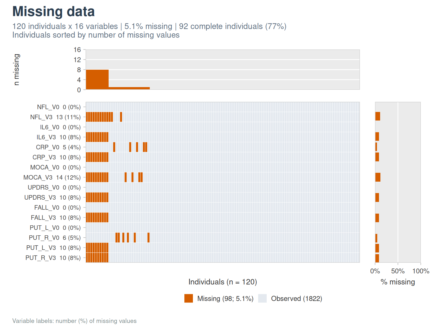
Normality
describe_normality(cohort_sim, c(AGE, BMI, NFL_V0, IL6_V0, CRP_V0, MOCA_V0), labels = labs)
#> # A tibble: 6 × 9
#>   Variable Label           N     W p_Shapiro     p_AD Skewness Kurtosis Verdict
#>   <chr>    <chr>       <int> <dbl>     <dbl>    <dbl>    <dbl>    <dbl> <chr>
#> 1 AGE      Age (years)   120 0.989  4.37e- 1 2.12e- 1  -0.0891    0.229 Compati…
#> 2 BMI      BMI           116 0.987  3.47e- 1 6.55e- 1  -0.192    -0.354 Compati…
#> 3 NFL_V0   NfL V0        120 0.808  3.08e-11 1.49e-10   2.48     10.5   Strong …
#> 4 IL6_V0   IL-6 V0       120 0.712  4.97e-14 3.7 e-24   2.48      7.04  Strong …
#> 5 CRP_V0   CRP V0        115 0.589  2.00e-16 3.7 e-24   3.93     20.2   Strong …
#> 6 MOCA_V0  MoCA V0       120 0.947  1.22e- 4 1.16e- 4  -0.335    -0.561 Slight …
plot_distribution_overview(cohort_sim, c(AGE, BMI, NFL_V0, IL6_V0, CRP_V0, MOCA_V0, UPDRS_V0), labels = labs)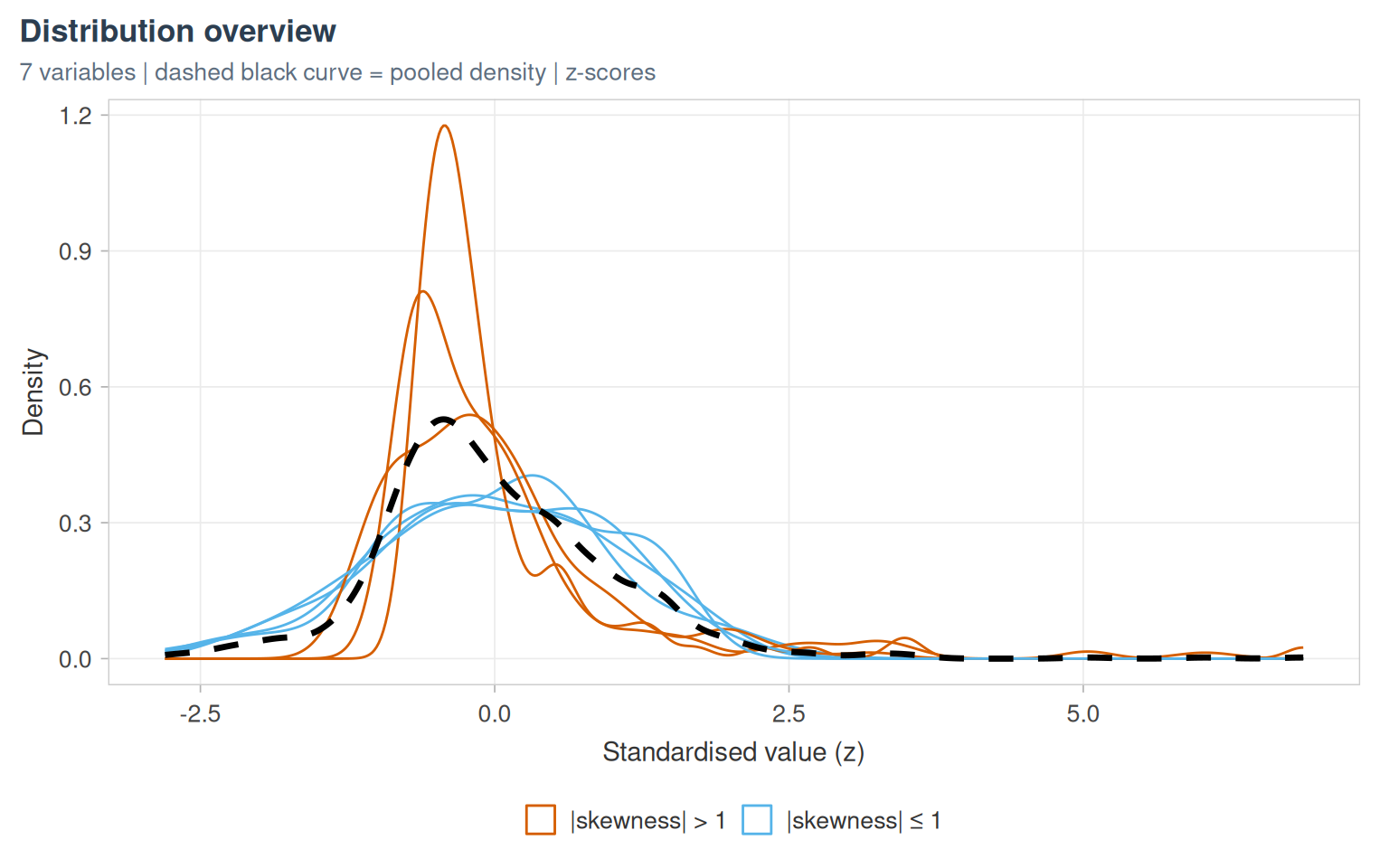
Correlations
cm <- cor_matrix_test(cohort_sim, c(AGE, BMI, NFL_V0, IL6_V0, CRP_V0, MOCA_V0, UPDRS_V0))
plot_cor_heatmap(cm, labels = labs)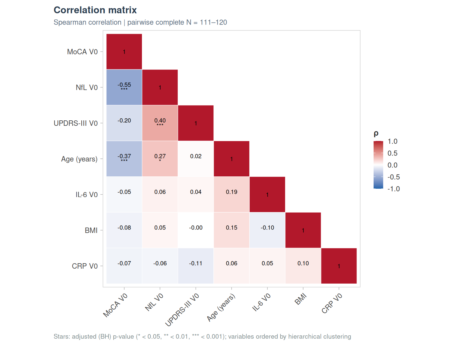
Partial correlations, adjusted for age and sex:
cc <- plot_cor_cross(cohort_sim, c(NFL_V0, IL6_V0, CRP_V0), c(MOCA_V0, UPDRS_V0),
                     covariates = c(AGE, SEX), labels = labs)
cc$plot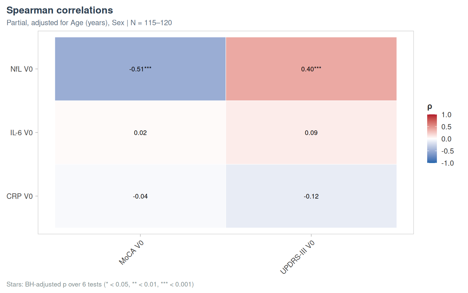
Principal component analysis
pc <- pca_compute(cohort_sim, c(AGE, BMI, NFL_V0, IL6_V0, CRP_V0, MOCA_V0, UPDRS_V0), id_col = ID,
                  impute = "median")
plot_pca_scree(pc)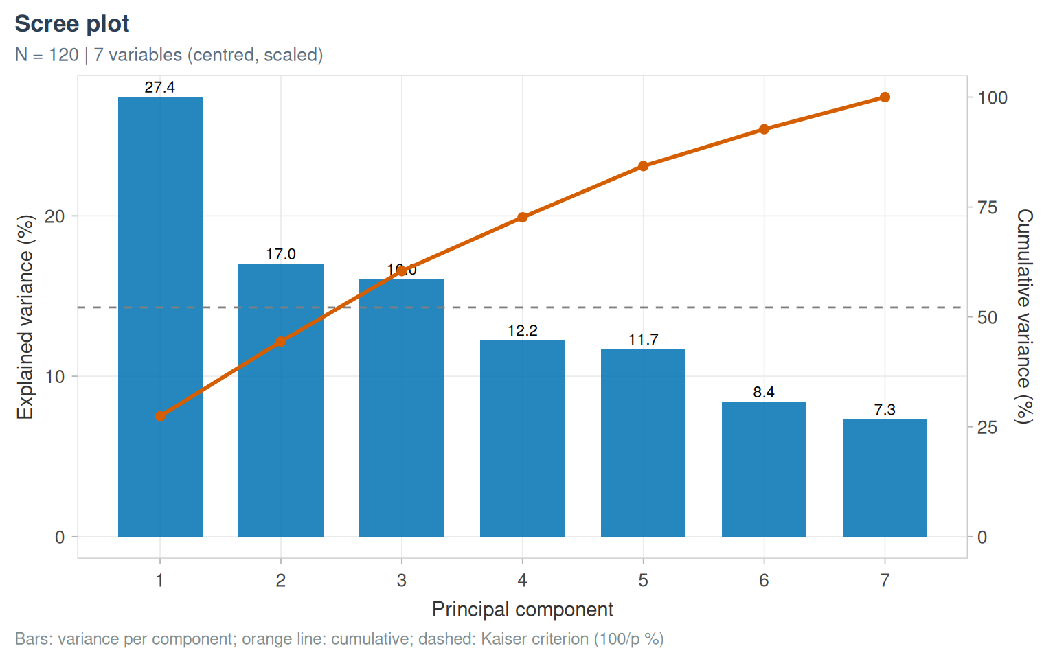
plot_pca_ind(pc, cohort_sim, id_col = ID, color_var = GROUP, labels = labs)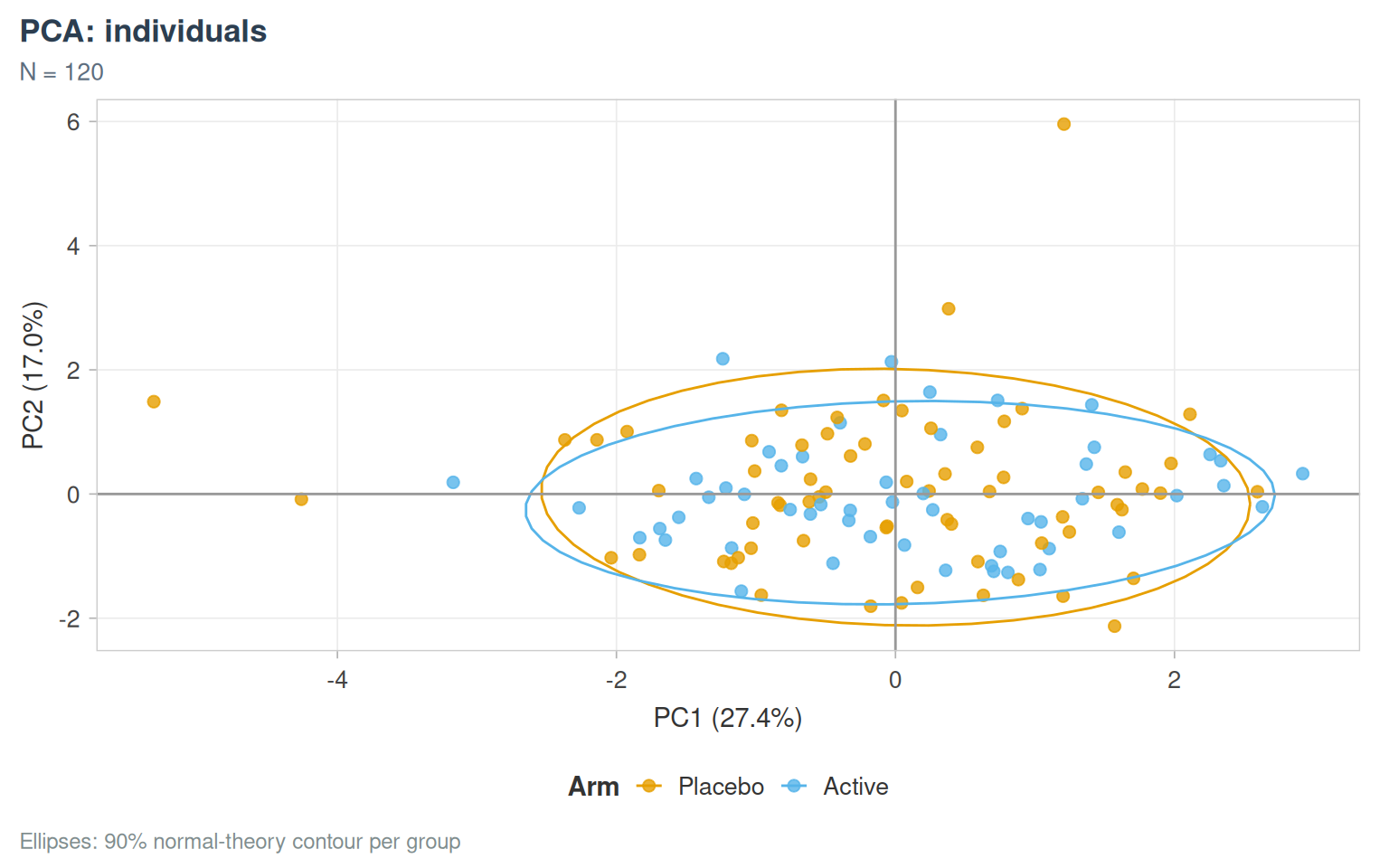
plot_pca_var(pc, labels = labs, groups = list(Biomarkers = c("NFL_V0", "IL6_V0", "CRP_V0"),
                                              Clinical = c("MOCA_V0", "UPDRS_V0")))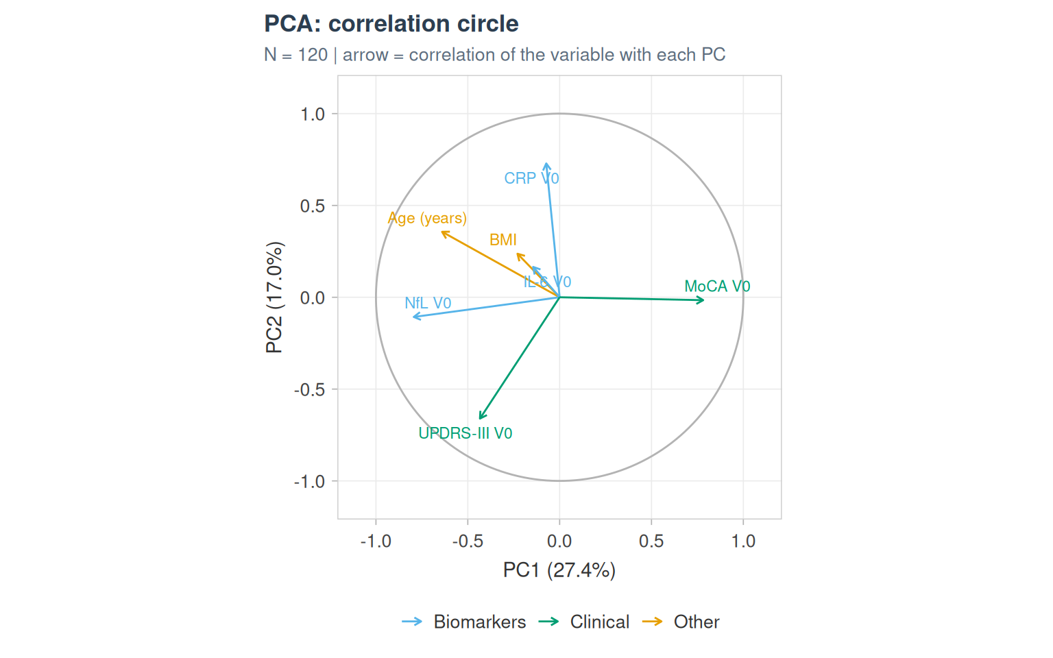
plot_pca_contrib(pc, axes = 1:2, labels = labs)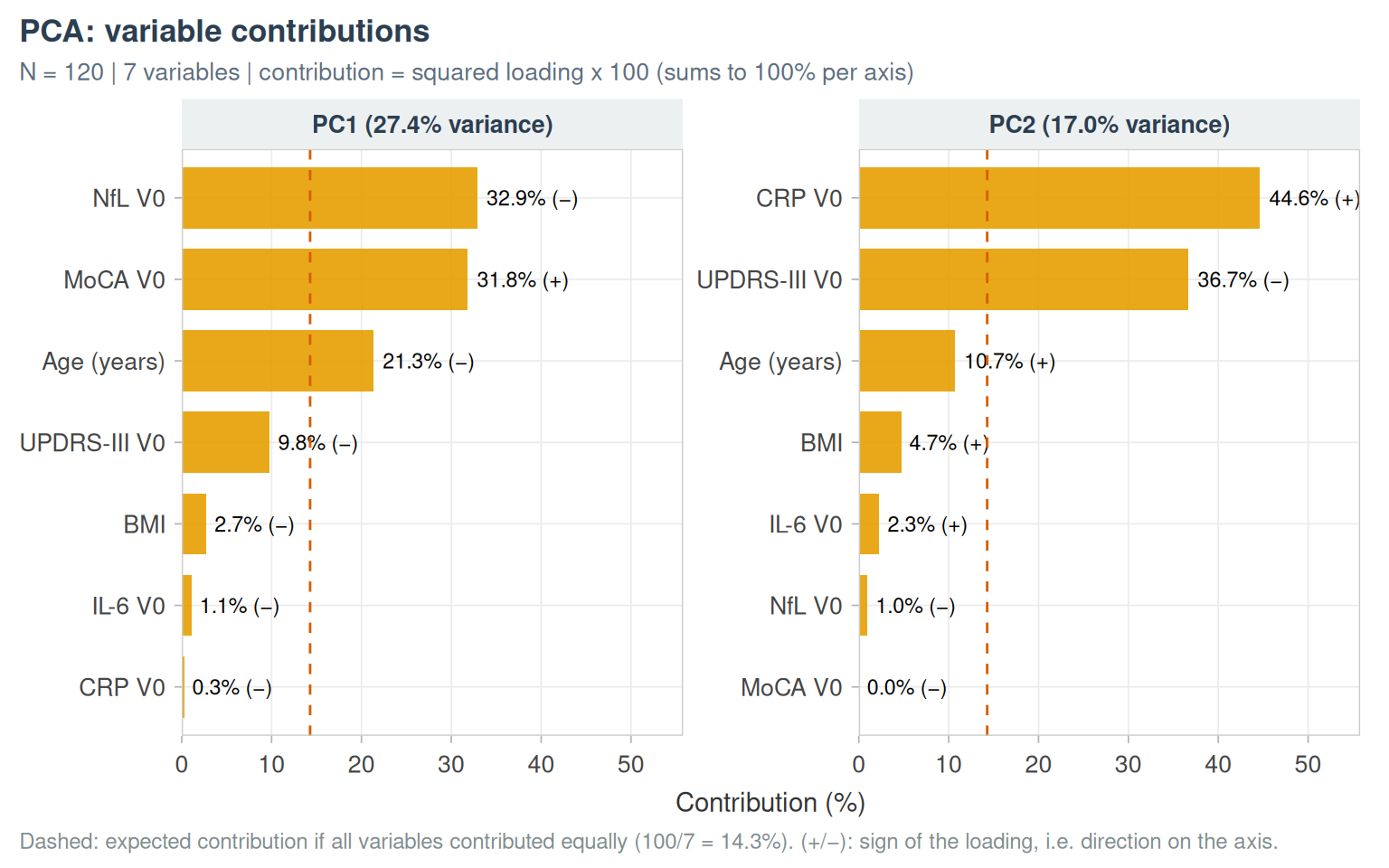
Changes between visits
plot_paired_visits(cohort_sim, c(NFL_V0, MOCA_V0), id_col = ID, labels = labs, transitions = TRUE)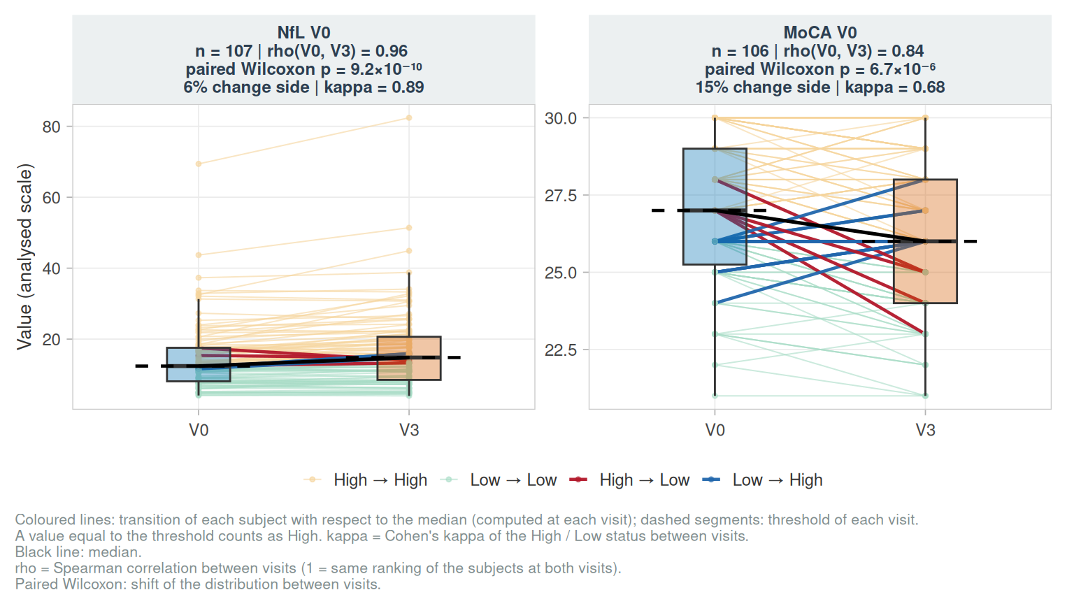
The reclassification table of categorised variables between visits is lodestar::cut_transition_table().