Show the code
# Données
library(dplyr)        # manipulation des données

# Esthétique
library(latex2exp)   ## TeX
library(ggplot2) ## ggplot# Données
library(dplyr) # manipulation des données
# Esthétique
library(latex2exp) ## TeX
library(ggplot2) ## ggplotSim_AR2 <- function(n, a, b) {
eps <- rnorm(n + 100)
x <- rnorm(n + 100)
for (i in (3:(n + 100))) {
x[i] <- eps[i] - a * x[i - 1] - b * x[i - 2]
}
ar2 <- x[101:(n + 100)]
return(ts(ar2))
}ggTimeSerie <- function(ts, main_title = NULL) {
df_series <- data.frame(Time = as.numeric(time(ts)), TimeSerie = ts)
colnames(df_series) <- c("Time", "TimeSerie")
if(is.null(main_title)){
main <- latex2exp::TeX(paste0("Série $( x_t )_{t=0, ...,n}$ avec n = ", length(ts)))
} else
main <- latex2exp::TeX(main_title)
p <- ggplot(df_series, aes(x = Time, y = TimeSerie)) +
geom_line(color = "red") +
labs(title = main,
x = "Time",
y = "Simulated series") +
theme_minimal()
if(length(time(ts(ts))) == length(ts)){
p <- p
} else
p <- p +
scale_x_continuous(
breaks = seq(floor(min(df_series$Time)), ceiling(max(df_series$Time)), by = 2),
labels = function(x) floor(x)
)
return(p)
}ggACF <- function(ts) {
acf_data <- acf(ts, plot = FALSE)
df_acf <- data.frame(Lag = acf_data$lag, ACF = acf_data$acf)
pacf_data <- pacf(ts, plot = FALSE)
df_pacf <- data.frame(Lag = pacf_data$lag, PACF = pacf_data$acf)
# Intervalle de confiance
ci <- qnorm((1 + 0.95) / 2) / sqrt(length(ts))
# ACF
p_acf <- ggplot(df_acf, aes(x = Lag, y = ACF)) +
geom_segment(aes(xend = Lag, yend = 0), color = "red") +
geom_point(color = "red") +
labs(title = "Autocorrelation Function (ACF)", x = "Lag", y = "ACF") +
geom_hline(yintercept = c(-ci, ci), color = "blue", linetype = "dashed") +
theme_minimal()
# PACF
p_pacf <- ggplot(df_pacf, aes(x = Lag, y = PACF)) +
geom_segment(aes(xend = Lag, yend = 0), color = "red") +
geom_point(color = "red") +
labs(title = "Partial Autocorrelation Function (PACF)", x = "Lag", y = "PACF") +
geom_hline(yintercept = c(-ci, ci), color = "blue", linetype = "dashed") +
theme_minimal()
return(list(ACF = p_acf, PACF = p_pacf))
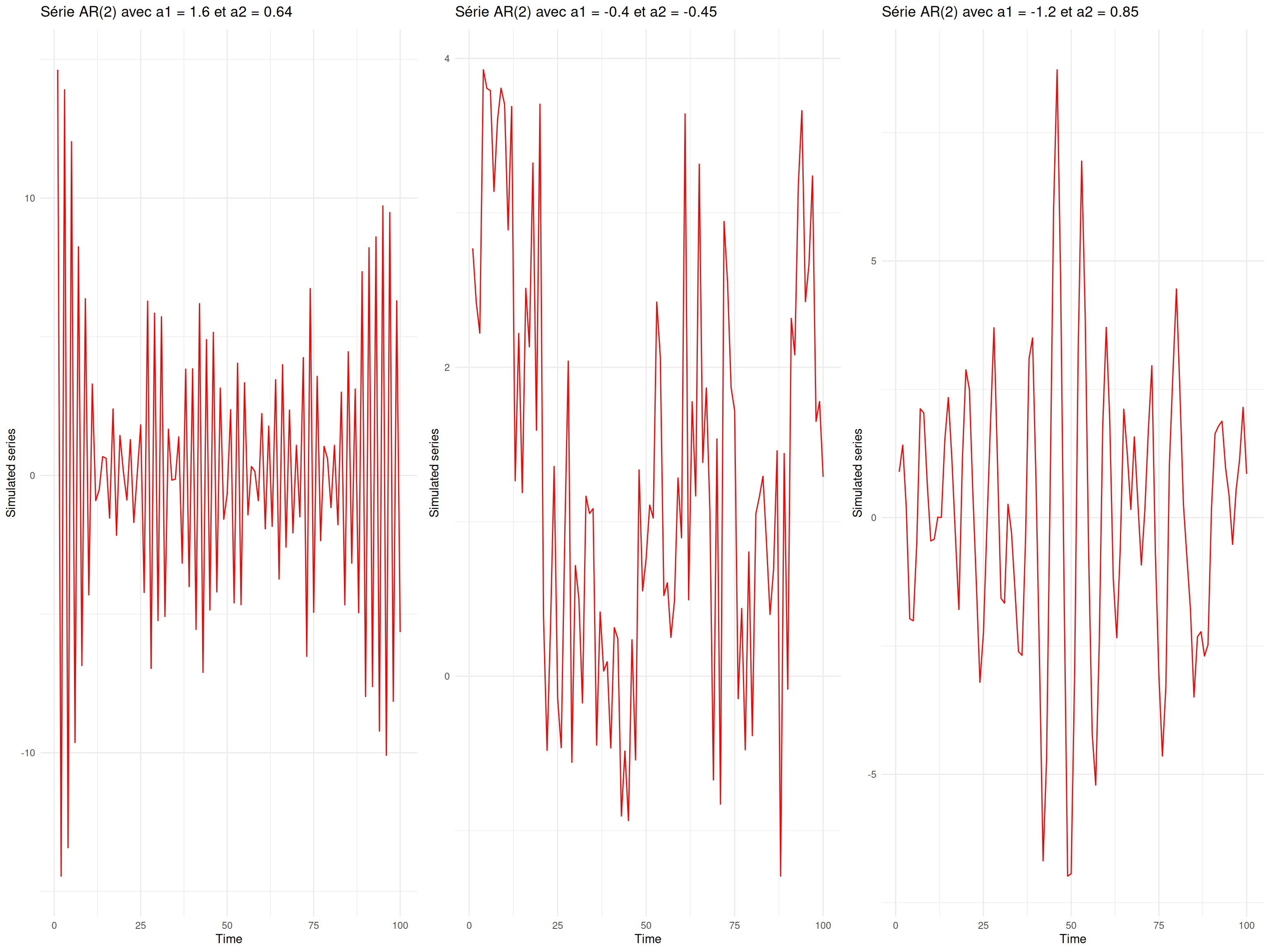
}set.seed(140400)Dans cette exo nous allons travailler sur 3 modèles du type AR(2) avec des coefficient +,+ ou -, - ou +, -.
\(X_t + 1.6X_{t-1} + .64X_{t-2} = w_t\)
\(X_t - .4X_{t-1} - .45X_{t-2} = w_t\)
\(X_t - 1.2X_{t-1} + .85X_{t-2} = w_t\)
n <- 100
a1 <- c(1.6, -0.4, -1.2)
a2 <- c(0.64, -0.45, 0.85)

gridExtra::grid.arrange(
  ggTimeSerie(
    Sim_AR2(n, a1[1], a2[1]),
    main_title = paste0("Série AR(2) avec a1 = ", a1[1], " et a2 = ", a2[1])
  ),
  ggTimeSerie(
    Sim_AR2(n, a1[2], a2[2]),
    main_title = paste0("Série AR(2) avec a1 = ", a1[2], " et a2 = ", a2[2])
  ),
  ggTimeSerie(
    Sim_AR2(n, a1[3], a2[3]),
    main_title = paste0("Série AR(2) avec a1 = ", a1[3], " et a2 = ", a2[3])
  ),
  ncol = 3
)
Pour les trois modèles AR(2) décrits ci-dessus, déterminer l’équations de récurrence satisfaite par ACF \(\rho\) et donner la solution (en précisant toutes les constantes)
Nous allons maintenant utiliser les résultats théoriques précédents pour tracer les valeurs des l’ACF \(\rho(h))\) pour \(h = 1...2\). Vérifier vos résultats en utilisant la fonction ARMAacf
sessioninfo::session_info(pkgs = "attached")─ Session info ───────────────────────────────────────────────────────────────
setting value
version R version 4.4.2 (2024-10-31)
os Ubuntu 24.04.1 LTS
system x86_64, linux-gnu
ui X11
language (EN)
collate fr_FR.UTF-8
ctype fr_FR.UTF-8
tz Europe/Paris
date 2025-03-07
pandoc 3.2 @ /usr/lib/rstudio/resources/app/bin/quarto/bin/tools/x86_64/ (via rmarkdown)
─ Packages ───────────────────────────────────────────────────────────────────
package * version date (UTC) lib source
dplyr * 1.1.4 2023-11-17 [1] CRAN (R 4.4.2)
ggplot2 * 3.5.1 2024-04-23 [1] CRAN (R 4.4.2)
latex2exp * 0.9.6 2022-11-28 [1] CRAN (R 4.4.2)
[1] /home/clement/R/x86_64-pc-linux-gnu-library/4.4
[2] /usr/local/lib/R/site-library
[3] /usr/lib/R/site-library
[4] /usr/lib/R/library
──────────────────────────────────────────────────────────────────────────────Tracer les valeurs des l’ACF \(\rho(h)\) pour \(h = 1, 2\) . Vérifier vos résultats en utilisant la fonction ARMAacf.
# On pose nos paramètres
a1 = c(1.6, -0.4, -1.2)
a2 = c(0.64, -0.45, 0.85)ARMAacf(ar = c(-a1[1], -a2[1]), ma = 0, lag.max = 2, pacf = FALSE) 0 1 2
1.0000000 -0.9756098 0.9209756 ARMAacf(ar = c(-a1[2], -a2[2]), ma = 0, lag.max = 2, pacf = FALSE) 0 1 2
1.0000000 0.7272727 0.7409091 ARMAacf(ar = c(-a1[3], -a2[3]), ma = 0, lag.max = 2, pacf = FALSE) 0 1 2
1.00000000 0.64864865 -0.07162162 # lag.max = n fait calculer et afficher les n premières valeurs en partant de 0Pour \(h = 1, 2\) on retrouve bien les valeurs calculées à la question 1.
On se propose de Généraliser en comparant les fonctions calculés en question 1 avec ARMAacf et la fonction acf de r, \(\forall h\).
# On code notre fonction AR(2)
n = 100


AR2 = function(n, a, b) {
  eps = rnorm(n + 100)
  x = rnorm(n + 100) #c'est pour donner la taille mais après on remplacera toute les valeurs
  # on suppose que X_0 est une rnorm
  for (i in (3:(n + 100))) {
    x[i] = eps[i] - a * x[i - 1] - b * x[i - 2]
  }
  X_final = x[101:(n + 100)]
  return(X_final)
}
# On code des fonction pour définir \rho à partir des calculs de la question 1

rho1 = function(h){
  r = (-5/4)^(-h) * (1 + h * (9/41))
  return(r)
}

rho2 = function(h){
  r = (135/154) * (9/10)^h + (19/154) * (-1)^h * (1/2)^h
  return(r)
}

rho3 = function(h){
  mod_z1 = sqrt(340/289)
  arg_z1 = atan(7/6)
  A = ( ( (24/37) * sqrt(30/17) - cos(atan(7/6)) / sin(atan(7/6))) )^2
  c1 = -sqrt(1+A)
  c2 = acos(1/c1)
  r = c1 * mod_z1^(-h) * cos(h * arg_z1 + c2)
  return(r)
}


