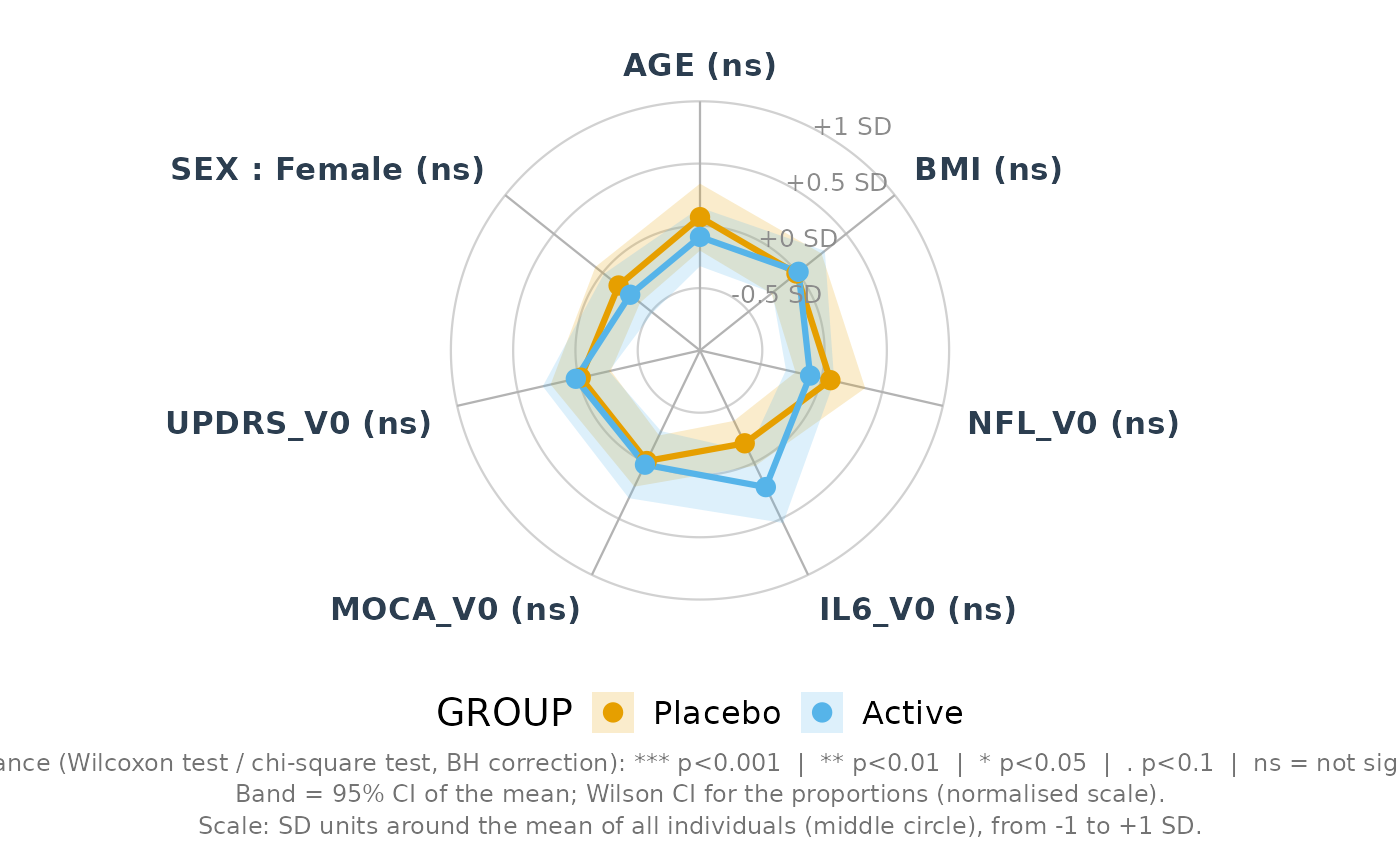
Each numeric variable gives one axis (mean or median per group); each categorical variable gives one or several axes (proportion of a level per group). Every value is brought to a 0-100% scale (configurable normalisation) with an optional confidence band. A between-group test per axis (Wilcoxon / Kruskal-Wallis / t / ANOVA / chi-squared / Fisher), with a multiplicity correction, adds stars or p-values to the labels.
Usage
plot_radar(
  data,
  vars,
  group = NULL,
  group_levels = NULL,
  group_labels = NULL,
  labels = NULL,
  var_order = NULL,
  reverse = NULL,
  force_quali = NULL,
  quali_levels = NULL,
  quali_expand = TRUE,
  quali_sep = " : ",
  stat = c("mean", "median"),
  ci = TRUE,
  ci_level = 0.95,
  ci_method = c("t", "boot", "se", "sd"),
  n_boot = 1000,
  seed = NULL,
  normalize = c("minmax", "quantile", "summary", "zscore", "rank", "none"),
  limits = NULL,
  reference = NULL,
  z_range = c(-1, 1),
  quantile_probs = c(0.025, 0.975),
  normalize_quali = FALSE,
  clip = TRUE,
  test = c("auto", "wilcox", "kruskal", "t", "anova", "none"),
  test_quali = c("auto", "chisq", "fisher", "none"),
  p_adjust = "BH",
  show_signif = TRUE,
  p_values = NULL,
  test_label = NULL,
  signif_format = c("stars", "p", "both"),
  signif_cutpoints = c(0.001, 0.01, 0.05, 0.1),
  signif_symbols = c("***", "**", "*", ".", "ns"),
  p_digits = 3,
  start_angle = 90,
  clockwise = TRUE,
  inner_radius = 0,
  grid_levels = c(0.25, 0.5, 0.75, 1),
  grid_shape = c("circle", "polygon"),
  grid_colour = "grey82",
  grid_linewidth = 0.4,
  grid_linetype = "solid",
  spoke_colour = "grey70",
  spoke_linewidth = 0.4,
  background_fill = NA,
  show_grid_labels = TRUE,
  grid_label_fmt = NULL,
  grid_label_angle = NULL,
  grid_label_size = 3.3,
  grid_label_colour = "grey55",
  palette = "okabe",
  colours = NULL,
  line_width = 1.1,
  linetypes = NULL,
  point_size = 2.8,
  point_shape = 19,
  show_points = TRUE,
  band_alpha = 0.2,
  fill_alpha = 0,
  show_values = FALSE,
  value_digits = 1,
  value_size = 3,
  label_size = 4.2,
  label_colour = "#2C3E50",
  label_fontface = "bold",
  label_offset = 0.1,
  label_wrap = NULL,
  label_lineheight = 0.9,
  title = NULL,
  subtitle = NULL,
  caption = NULL,
  legend_title = NULL,
  legend_position = "bottom",
  legend_nrow = NULL,
  show_legend = NULL,
  base_size = 13,
  base_family = "",
  title_size = NULL,
  caption_size = 9,
  plot_margin = c(10, 20, 10, 20),
  expand_x = 0.65,
  expand_y = 0.2,
  return_data = FALSE
)
Arguments
- data
Wide data frame, one row per subject.
- vars
Variables on the radar (names or tidyselect). Numeric: quantitative axes; factor / character / logical: proportions.
- group
Grouping column (
NULL: one profile).- group_levels
Order of the groups.
- group_labels
Renaming of the groups (named
old = new, or unnamed in level order).- labels
Axis labels: named vector (variable name, or
"variable:level"for a categorical axis) or unnamed vector of one label per axis.- var_order
Order of the axes (variable names, axis ids or labels), starting at
start_angle; axes not listed follow.- reverse
Variables reversed (1 - x), e.g. when "higher = better" for some scales and not others.
- force_quali
Numeric variables treated as categorical (e.g. 0/1).
- quali_levels
Named list: level(s) shown for each categorical variable, e.g.
list(SEX = "Female"). Default:TRUEfor a logical, the 2nd level of a binary variable, every level otherwise.- quali_expand
If
FALSE, a variable with more than 2 levels and noquali_levelsgives a single axis (1st level).- quali_sep
Separator of the
"variable : level"labels.- stat
"mean"or"median".- ci
Draw the confidence band.
- ci_level
Level of the confidence band.
- ci_method
"t"(Student CI),"boot"(percentile bootstrap),"se"(+/- 1 SE) or"sd"(+/- 1 SD). For the median,"t"and"se"switch to"boot". Proportions always use the Wilson CI.- n_boot
Number of bootstrap resamples.
- seed
Seed of the bootstrap and simulated Fisher tests (
NULL: the current random state is used; with a seed, the random state is restored afterwards).- normalize
"minmax"(individual data),"quantile"(same on thequantile_probsquantiles, robust to extremes),"summary"(min-max of the group summaries),"zscore"(SD units around the mean ofreference, 50% = reference mean, edges =z_rangeSD; recommended when group differences are small compared with the range),"rank"(percentile ranks of the subjects, all groups pooled, then mean per group) or"none"(data assumed in [0, 1]).- limits
Named list of fixed bounds per variable, with priority, e.g.
list(MOCA_V0 = c(0, 30))(advised for bounded clinical scales).- reference
Reference group of
normalize = "zscore"(NULL: all subjects).- z_range
Range shown in SD units for
"zscore".- quantile_probs
Bounds of
normalize = "quantile".- normalize_quali
Normalise the proportions too (
FALSE: shown as is, 0-100%).- clip
Clip the normalised values to [0, 1].
- test
Quantitative axes:
"auto"(Wilcoxon with 2 groups, Kruskal-Wallis otherwise),"wilcox","kruskal","t"(Welch t / Welch ANOVA),"anova"or"none".- test_quali
Categorical axes:
"auto"(chi-squared, or Fisher with expected counts < 5),"chisq","fisher"or"none".- p_adjust
Method of
stats::p.adjust().- show_signif
Add the significance to the labels.
- p_values
P-values computed elsewhere (named by variable or axis id), e.g. paired tests between visits; they replace
testandtest_quali(p_adjustis applied to them).- test_label
Name of the test of
p_values, for the caption.- signif_format
"stars","p"or"both".- signif_cutpoints, signif_symbols
Cut-points and symbols of the stars (
length(signif_symbols) == length(signif_cutpoints) + 1, the last symbol meaning "not significant").- p_digits
Decimals of the p-values shown.
- start_angle
Angle of the first axis, in degrees (90 = top).
- clockwise
Direction of the axes.
- inner_radius
Radius of the central hole (0 to < 1), so that small values are not squashed at the centre.
- grid_levels
Levels of the grid circles, on [0, 1].
- grid_shape
"circle"or"polygon"(spider web).- grid_colour, grid_linewidth, grid_linetype
Style of the grid.
- spoke_colour, spoke_linewidth
Style of the spokes.
- background_fill
Fill of the disc (
NA: none).- show_grid_labels
Print the grid levels.
- grid_label_fmt
Function formatting the grid levels (
NULL: automatic, %, SD for"zscore", percentiles for"rank").- grid_label_angle
Angle where the grid levels are printed (default:
start_angle).- grid_label_size, grid_label_colour
Style of the grid levels.
- palette
Palette of the groups (see
pal_levels()); default"okabe".- colours
Explicit colours (named by group or not), with priority.
- line_width
Width of the profiles.
- linetypes
Line types per group (
NULL: solid).- point_size
Size of the points.
- point_shape
Shape of the points (one value, or one per group).
- show_points
Draw the points.
- band_alpha
Transparency of the confidence band.
- fill_alpha
Fill of the profile areas (0 = none).
- show_values
Print the raw (non-normalised) value at each point.
- value_digits, value_size
Format of the values printed.
- label_size, label_colour, label_fontface
Style of the axis labels.
- label_offset
Distance between the labels and the outer circle.
- label_wrap
Width (characters) for wrapping the labels (
NULL: no wrapping).- label_lineheight
Line height of multi-line labels.
- title, subtitle
Titles.
- caption
NULL= automatic caption (tests and CI),FALSE= none, or a text.- legend_title
Title of the legend (default: name of
group).- legend_position
"bottom","right","top","left"or"none".- legend_nrow
Number of rows of the legend.
- show_legend
NULL= automatic (hidden with a single group).- base_size, base_family
Base font size and family.
- title_size, caption_size
Sizes of the title and caption.
- plot_margin
Margins
c(top, right, bottom, left)in points.- expand_x, expand_y
Space around the radar for the labels.
- return_data
TRUE: returnlist(plot, summary, tests).