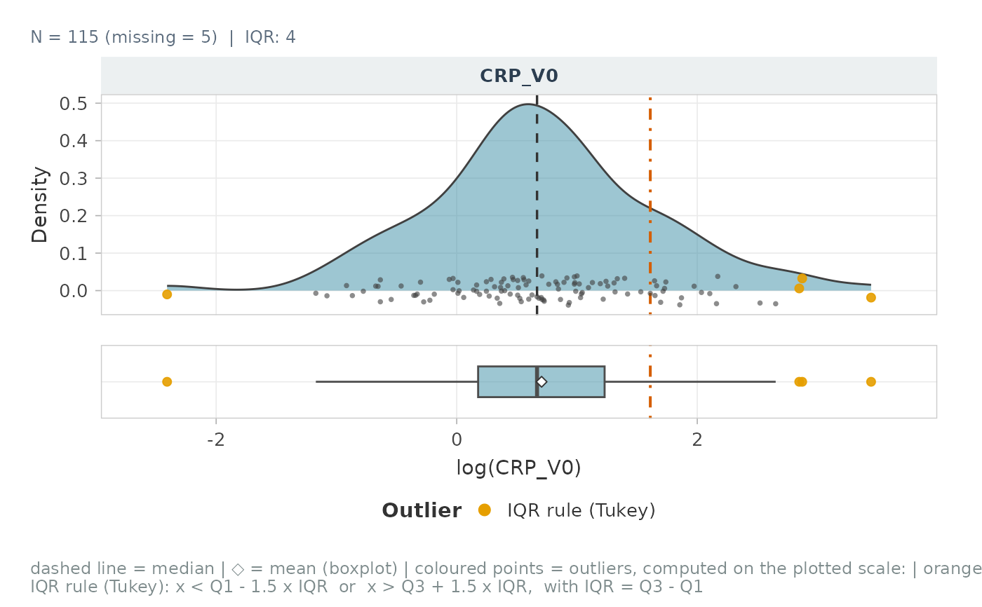
Distribution of one or several variables — plot

One panel per variable, its type chosen from the data:

continuous: density, jittered points (rug) and an aligned horizontal boxplot;
discrete (integer scores such as MoCA or UPDRS): histogram with bin width 1 (a smoothed density would invent values);
categorical or binary: bar chart with N and %.

Usage

plot_distribution(
  data,
  vars = NULL,
  group = NULL,
  metadata = NULL,
  id_col = NULL,
  labels = NULL,
  type = "auto",
  discrete_max = 15,
  transform = NULL,
  outlier_mad = FALSE,
  outlier_iqr = TRUE,
  mad_z_threshold = 3.5,
  iqr_k = 1.5,
  show_points = TRUE,
  show_box = TRUE,
  show_stats = c("median"),
  ref_lines = NULL,
  ref_label = "reference line",
  test = c("auto", "nonparametric", "parametric", "none"),
  palette = NULL,
  fill_color = "#3B8EA5",
  value_label = NULL,
  ncol = 3,
  base_size = 11,
  rug_height_pct = 0.08,
  heights = c(3, 1),
  title = NULL,
  subtitle = NULL,
  seed = 1
)

Arguments

data: A data frame, tibble or matrix.
vars: Variables to plot (names or tidyselect; default: all but the identifier and the group).
group: Optional grouping column, in data or in metadata.
metadata: Optional data frame holding group, joined on id_col.
id_col: Identifier column (default: row names, or row numbers). Required with metadata.
labels: Optional named vector of labels.
type: "auto", "density", "histogram" or "bar", or a named vector variable -> type.
discrete_max: Integer variables with at most this many distinct values (or a range below three times this value) are drawn as histograms.
transform: NULL, "log", "log10", "log1p", "sqrt" or a function, applied for display only.
outlier_mad, outlier_iqr: Flag outliers with the MAD rule and / or Tukey's rule.
mad_z_threshold: Cut-off of the modified z-score.
iqr_k: Multiplier of the Tukey fences.
show_points: Show the jittered points under the density.
show_box: Add the horizontal boxplot under each panel.
show_stats: Subset of c("median", "mean"): vertical lines.
ref_lines: Numeric (every variable) or named list variable -> values.
ref_label: Legend text of the reference lines (caption).
test: "auto" / "nonparametric", "parametric" or "none".
palette: Colours of the groups (see pal_levels()).
fill_color: Fill colour without groups.
value_label: X-axis title (default: label of the variable).
ncol: Number of columns of panels.
base_size: Base font size.
rug_height_pct: Height of the jittered points, as a share of the density peak.
heights: Relative heights of the density and boxplot panels.
title, subtitle: Titles of the whole figure.
seed: Seed of the jitter.

Value

A patchwork with the attributes "outliers" (one row per flagged value) and "tests" (one row per variable with p_adj_BH), or NULL when nothing can be plotted.

Details

Options: groups (from data or joined from metadata), on-the-fly display transformation, outliers flagged by the MAD and / or IQR rules (see outlier_flag_mad(), computed on the plotted scale, coloured by the rule that flags them, formulas printed in the caption), a group test in each subtitle (Wilcoxon / Kruskal-Wallis, Welch t / ANOVA, Fisher / chi-squared) and reference lines per variable (LOD, clinical cut-off...).

Examples

p <- plot_distribution(cohort_sim, c(NFL_V0, MOCA_V0, SEX), group = GROUP,
                       outlier_mad = TRUE)
p

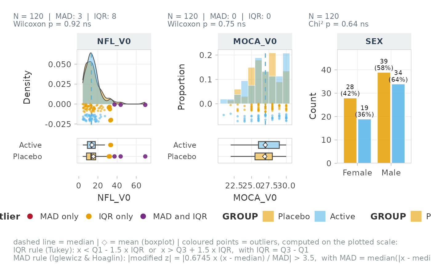attr(p, "tests")
#> # A tibble: 3 × 4
#>   Variable Test         p p_adj_BH
#>   <chr>    <chr>    <dbl>    <dbl>
#> 1 NFL_V0   Wilcoxon 0.924    0.924
#> 2 MOCA_V0  Wilcoxon 0.747    0.924
#> 3 SEX      Chi²     0.636    0.924
plot_distribution(cohort_sim, CRP_V0, transform = "log", ref_lines = list(CRP_V0 = log(5)))