---
title: "Survival Analysis: From Censoring to the Cox Model"
author: "Clément Poupelin"
date: 07-13-2026
date-modified: "`r Sys.Date()`"
bibliography: references.bib
format:
html:
embed-resources: false
toc: true
code-fold: true
code-summary: "Show the code"
code-tools: true
toc-location: right
page-layout: article
code-overflow: wrap
number-sections: false
editor: visual
categories: ["Survival Analysis", "Biostatistics"]
description: "Introduction to survival analysis: censoring, the Kaplan-Meier estimator, the log-rank test and the Cox proportional hazards model, with a full R application."
execute:
echo: true
warning: false
message: false
error: true
---
## Setup
::: panel-tabset
### packages
```{r}
library(dplyr)      ## Data manipulation
library(tidyr)      ## Data manipulation
library(ggplot2)     ## Plots
library(viridis)     ## Colorblind palette

library(survival)    ## Core survival analysis (Surv, survfit, coxph, survdiff)
library(survminer)   ## ggplot2-based survival curves (ggsurvplot, ggforest)
library(broom)       ## Tidy model outputs
library(knitr)       ## Tables
library(kableExtra)  ## Table styling
```
### Functions
```{r}
## Consistent ggplot2 theme used across every figure in the report, for a
## cleaner, more "modern article" look than the ggplot2/survminer defaults.
theme_survival <- function(base_size = 13) {
  theme_minimal(base_size = base_size, base_family = "sans") +
    theme(
      plot.title = element_text(face = "bold", size = rel(1.15), margin = margin(b = 6)),
      plot.subtitle = element_text(color = "grey35", margin = margin(b = 10)),
      axis.title = element_text(face = "bold", size = rel(0.95)),
      axis.text = element_text(color = "grey25"),
      panel.grid.minor = element_blank(),
      panel.grid.major = element_line(color = "grey90", linewidth = 0.3),
      legend.position = "top",
      legend.title = element_text(face = "bold"),
      strip.text = element_text(face = "bold", size = rel(1)),
      plot.margin = margin(10, 15, 10, 10)
    )
}

## Wraps broom::tidy() around a coxph object to build a publication-ready
## hazard-ratio table (estimate, HR, 95% CI, p-value), used throughout the
## report so that every number displayed is computed at render time rather
## than typed by hand.
cox_table <- function(fit, caption = NULL) {
  broom::tidy(fit, exponentiate = TRUE, conf.int = TRUE) %>%
    transmute(
      Term = term,
      `HR` = round(estimate, 3),
      `Std. Error` = round(std.error, 3),
      `95% CI` = paste0("[", round(conf.low, 3), " ; ", round(conf.high, 3), "]"),
      `p-value` = signif(p.value, 3)
    ) %>%
    kable(caption = caption) %>%
    kable_styling(full_width = FALSE)
}

## Modern ggplot2 forest plot of hazard ratios from a coxph object, used as
## a more visually consistent alternative to survminer::ggforest().
plot_forest <- function(fit, title = NULL) {
  broom::tidy(fit, exponentiate = TRUE, conf.int = TRUE) %>%
    mutate(term = reorder(term, estimate)) %>%
    ggplot(aes(x = estimate, y = term, color = estimate > 1)) +
    geom_vline(xintercept = 1, linetype = "dashed", color = "grey50") +
    geom_errorbarh(aes(xmin = conf.low, xmax = conf.high), height = 0.15, linewidth = 0.7) +
    geom_point(size = 3) +
    scale_x_log10() +
    scale_color_viridis_d(option = "D", begin = 0.15, end = 0.75, guide = "none") +
    labs(
      title = title,
      subtitle = "Hazard ratio and 95% confidence interval (log scale)",
      x = "Hazard ratio", y = NULL
    ) +
    theme_survival()
}

## Modern ggplot2 version of the Schoenfeld residual plot from a cox.zph
## object, used as a more visually consistent alternative to base
## plot(cox.zph(...)).
plot_schoenfeld <- function(zph) {
  as.data.frame(zph$y) %>%
    mutate(time = zph$x) %>%
    pivot_longer(-time, names_to = "Covariate", values_to = "Residual") %>%
    ggplot(aes(x = time, y = Residual)) +
    geom_hline(yintercept = 0, linetype = "dashed", color = "grey50") +
    geom_point(alpha = 0.35, color = viridis(1, begin = 0.25)) +
    geom_smooth(method = "loess", se = TRUE, color = "#B63679", fill = "#B6367933", linewidth = 0.8) +
    facet_wrap(~Covariate, scales = "free_y") +
    labs(
      title = "Schoenfeld residuals over time",
      subtitle = "A flat trend around zero supports the proportional hazards assumption",
      x = "Time", y = "Scaled residual"
    ) +
    theme_survival()
}
```
### Seed
```{r}
set.seed(140400)
```
:::
## Abstract
This tutorial provides a self-contained introduction to **survival analysis**, the branch of statistics dedicated to the modeling of time-to-event data under censoring.\
It covers the theoretical foundations together with a full applied illustration in `R` on the classic `lung` dataset from the `survival` package [@therneau2024survival].\
## Import Data
The dataset used in this report is the `lung` dataset, built into the `survival` package [@therneau2024survival]\
It contains survival data on patients with advanced lung cancer from the North Central Cancer Treatment Group [@loprinzi1994prospective].
```{r}
lung <- survival::lung

## The status variable is coded 1 = censored, 2 = dead in the raw dataset.
## We recode it to the conventional 0 = censored, 1 = event coding.
lung <- lung %>%
  mutate(
    status = recode(status, `1` = 0, `2` = 1),
    sex    = factor(sex, levels = c(1, 2), labels = c("Male", "Female")),
    ph.ecog = factor(ph.ecog)
  )
```
It includes `r nrow(lung)` individuals characterized by the `r ncol(lung)` following variables:
- `inst` : institution code
- `time` : survival time, in days
- `status` : event indicator (`0` = censored, `1` = death)
- `age` : age of the patient, in years
- `sex` : sex of the patient (`Male`, `Female`)
- `ph.ecog` : ECOG performance score rated by the physician, from `0` (asymptomatic) to `4` (bedridden)
- `ph.karno` : Karnofsky performance score rated by the physician (`0`-`100`)
- `pat.karno` : Karnofsky performance score rated by the patient (`0`-`100`)
- `meal.cal` : calories consumed at meals
- `wt.loss` : weight loss over the last six months, in pounds
```{r}
lung %>% DT::datatable()
```
::: {.callout-note}
For the applied part of this report, we keep the individuals with no missing value on the covariates used in the multivariate model.
```{r}
lung_cc <- lung %>%
  select(time, status, age, sex, ph.ecog, ph.karno, wt.loss) %>%
  na.omit()
```
:::
## Preliminary analysis
### Descriptive analysis
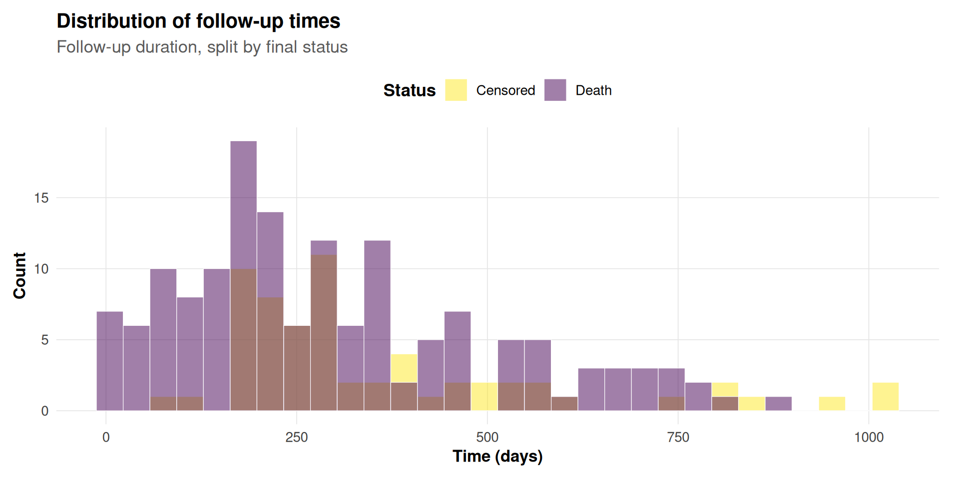
Before any modeling, it is essential to look at the **event / censoring balance** and the **distribution of follow-up times**, since these two elements drive the amount of information available for estimation.
::: {.callout-important title="What is censoring?"}
In a survival study, most participants are not observed until the event of interest actually happens. Some are still alive and event-free when the study ends, some drop out or are lost to follow-up, and some leave the study for reasons unrelated to the event under study.\
For all of these individuals, we only know that their true event time is **at least** as long as their observed follow-up time. So, we call this a **censored observation**.
This is fundamentally different from an ordinary missing value: we don't have *no* information, we have *partial* information ("this patient was still alive after day X"), and a correct analysis has to make use of that partial information rather than discard it or treat it as if the event had actually occurred.
:::
```{r, fig.width=10, fig.height=5}
lung_cc %>%
  mutate(status_lab = factor(status, levels = c(0, 1), labels = c("Censored", "Death"))) %>%
  ggplot(aes(x = time, fill = status_lab)) +
  geom_histogram(bins = 30, alpha = 0.5, color = "white", linewidth = 0.2, position = "identity") +
  scale_fill_viridis_d(option = "D", direction = -1) +
  labs(
    title = "Distribution of follow-up times",
    subtitle = "Follow-up duration, split by final status",
    x = "Time (days)", y = "Count", fill = "Status"
  ) +
  theme_survival()
```
```{r}
lung_cc %>%
  count(status) %>%
  mutate(status = ifelse(status == 1, "Death", "Censored"),
         proportion = round(n / sum(n), 3)) %>%
  kable(caption = "Table 1: Event / censoring balance in the analytic sample")
```
::: {.callout-tip}
Close to a third of the patients in the analytic sample are censored: their true survival time is only known to be **greater than** the last time they were observed.\
This censoring rate is exactly the kind of partial information described above, and is a central statistical difficulty.
:::
Before moving on, it is also worth checking the **balance of categorical covariates** that will later enter the Cox model — an imbalance here has direct consequences on how stable the corresponding hazard ratios will be.
```{r}
lung_cc %>%
  count(ph.ecog) %>%
  mutate(proportion = round(n / sum(n), 3)) %>%
  kable(caption = "Table 2: Number of patients per ECOG performance status level")
```
::: {.callout-warning title="A near-empty category"}
Only **one patient** in the analytic sample has `ph.ecog = 3` (the most severe level). A category this small cannot produce a stable hazard ratio or a meaningful Kaplan-Meier curve on its own: any model that treats it as a separate level will report a huge, essentially anecdotal effect for that category.
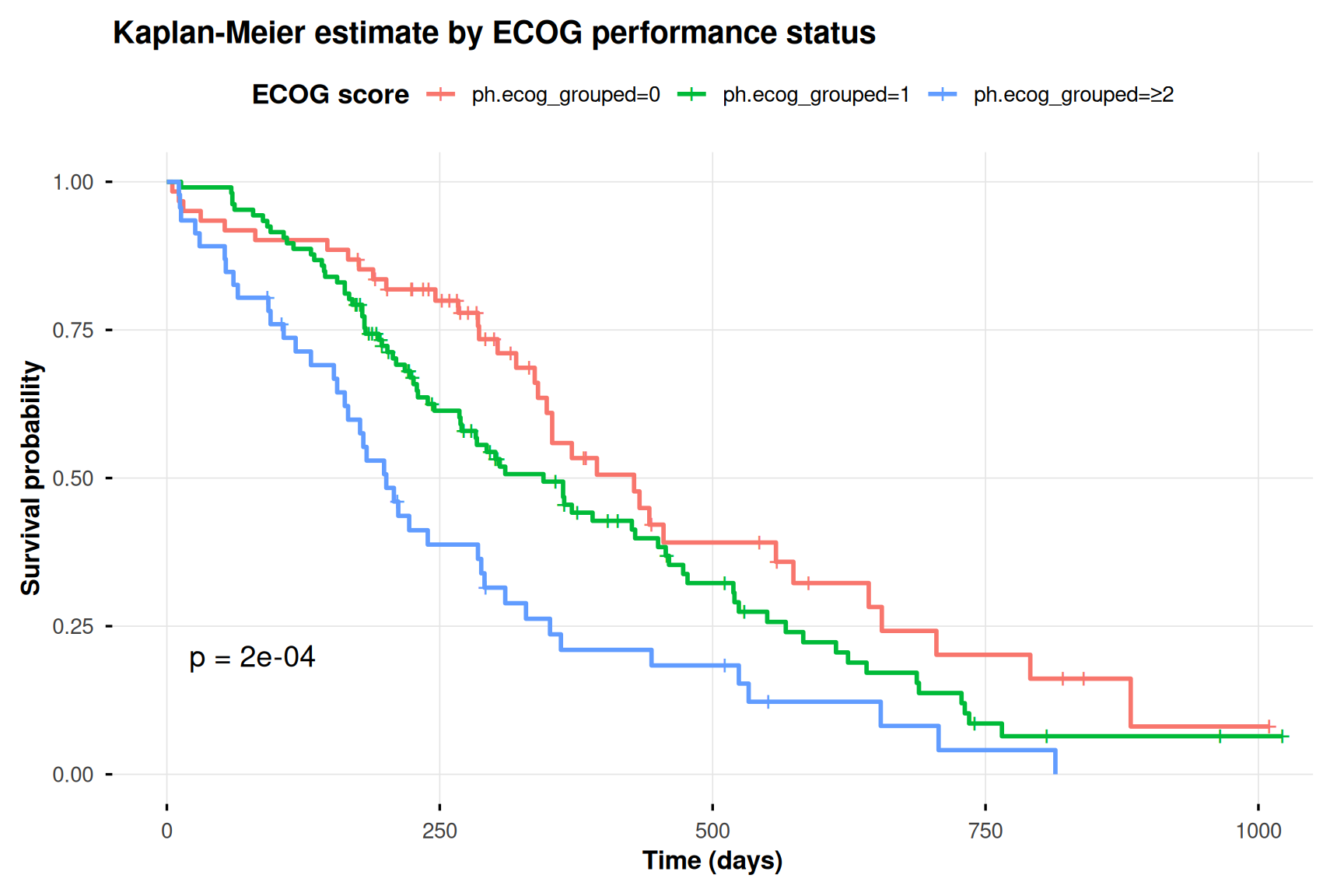
Rather than discarding this patient, we **regroup rare categories** for the modeling steps below: `ph.ecog = 2` and `ph.ecog = 3` are merged into a single "≥2" level, computed once here and reused throughout the rest of the report. The original four-level `ph.ecog` is kept for the descriptive Kaplan-Meier plot, where each observed trajectory is shown as-is.
:::
```{r}
lung_cc <- lung_cc %>%
  mutate(
    ph.ecog_grouped = factor(
      ifelse(ph.ecog %in% c("2", "3"), "\u22652", as.character(ph.ecog)),
      levels = c("0", "1", "\u22652")
    )
  )
```
### From standard regression to survival analysis
A natural first instinct would be to model `time` directly with a linear model, or to dichotomize the outcome ("dead within one year: yes/no") and use logistic regression. Both approaches fail for structural reasons:
- **Censoring is not missing data**: a censored observation still carries information. We know the patient survived *at least* until the censoring time. Removing censored individuals (a "complete case" analysis on `time`) or treating them as if they had the event at the censoring time both introduce **severe bias**, generally underestimating survival.
- **Dichotomizing the outcome throws away information**: reducing "died at day 40" and "died at day 400" to the same binary event discards the timing, which is precisely the quantity of interest.
- **The outcome is intrinsically dynamic**: what we want to model is not a single number but an entire function of time — the instantaneous risk of the event, which can vary as time passes.
**Survival analysis addresses these limitations by modeling directly the time-to-event distribution while formally accounting for censoring**, through the survival function and the hazard function introduced below.
## Theoretical foundations
### Time, event and censoring
Let $T$ be the (possibly unobserved) random variable representing the true time to the event of interest, and $C$ the random variable representing the censoring time. In the presence of **right censoring** (the most common case, and the one considered in this report), we observe for each individual $i$:
$$
\begin{cases}
\tilde{T}_i = \min(T_i, C_i) \\
\delta_i = \mathbb{1}\{T_i \leq C_i\}
\end{cases}
$$
where $\delta_i = 1$ if the event is observed ($T_i \leq C_i$) and $\delta_i = 0$ if the observation is censored ($T_i > C_i$).\
We generally assume **non-informative censoring**: conditional on the covariates, $T$ and $C$ are independent, so that censoring does not itself carry information about the risk of the event (this assumption is not testable from the data alone and must be justified by the study design).
::: {.callout-note collapse="true" title="Other types of censoring"}
- **Left censoring**: the event has already happened before the start of observation
- **Interval censoring**: the event occurred within a known window
These censorings are less common but follow the same overall logic; they are not developed further in this report.
:::
### Survival function and hazard function
The **survival function** gives the probability of being event-free beyond time $t$:
$$
S(t) = P(T > t)
$$
with $S(0) = 1$ and $S$ non-increasing. The **hazard function** (or instantaneous risk) gives the instantaneous rate of the event at $t$, conditional on having survived until $t$:
$$
h(t) = \lim_{\Delta t \to 0} \frac{P(t \leq T < t + \Delta t \mid T \geq t)}{\Delta t}
$$
Denoting $f(t) = -S'(t)$ the density of $T$, we have $h(t) = \dfrac{f(t)}{S(t)} = -\dfrac{S'(t)}{S(t)} = -\dfrac{d}{dt}\log S(t)$.
Integrating both sides between $0$ and $t$, and defining the **cumulative hazard function** $H(t) = \int_0^t h(u)\, du$:
$$
H(t) = \int_0^t h(u)\, du = -\big[\log S(u)\big]_0^t = -\log S(t) + \underbrace{\log S(0)}_{= 0}
$$
$$
\Leftrightarrow \boxed{S(t) = \exp\big(-H(t)\big)}
$$
This identity is central: it means that **estimating the hazard is equivalent to estimating the survival function**, which is exactly the strategy used by the Kaplan-Meier estimator and the Cox model below.
### Kaplan-Meier estimator
Let $t_{(1)} < t_{(2)} < \cdots < t_{(k)}$ be the **distinct** observed event times in the sample. At each $t_{(j)}$, denote:
- $n_j$ : the number of individuals still **at risk** just before $t_{(j)}$ (i.e. neither dead nor censored before $t_{(j)}$)
- $d_j$ : the number of events occurring exactly at $t_{(j)}$
The conditional probability of surviving past $t_{(j)}$, given that one has survived up to $t_{(j)}$, is estimated by $1 - d_j / n_j$. Because survival to time $t$ requires surviving *each* preceding interval in turn, the survival function is estimated as a **product of conditional probabilities** — hence the name "product-limit estimator":
$$
\hat{S}(t) = \prod_{j : t_{(j)} \leq t} \left(1 - \frac{d_j}{n_j}\right)
$$
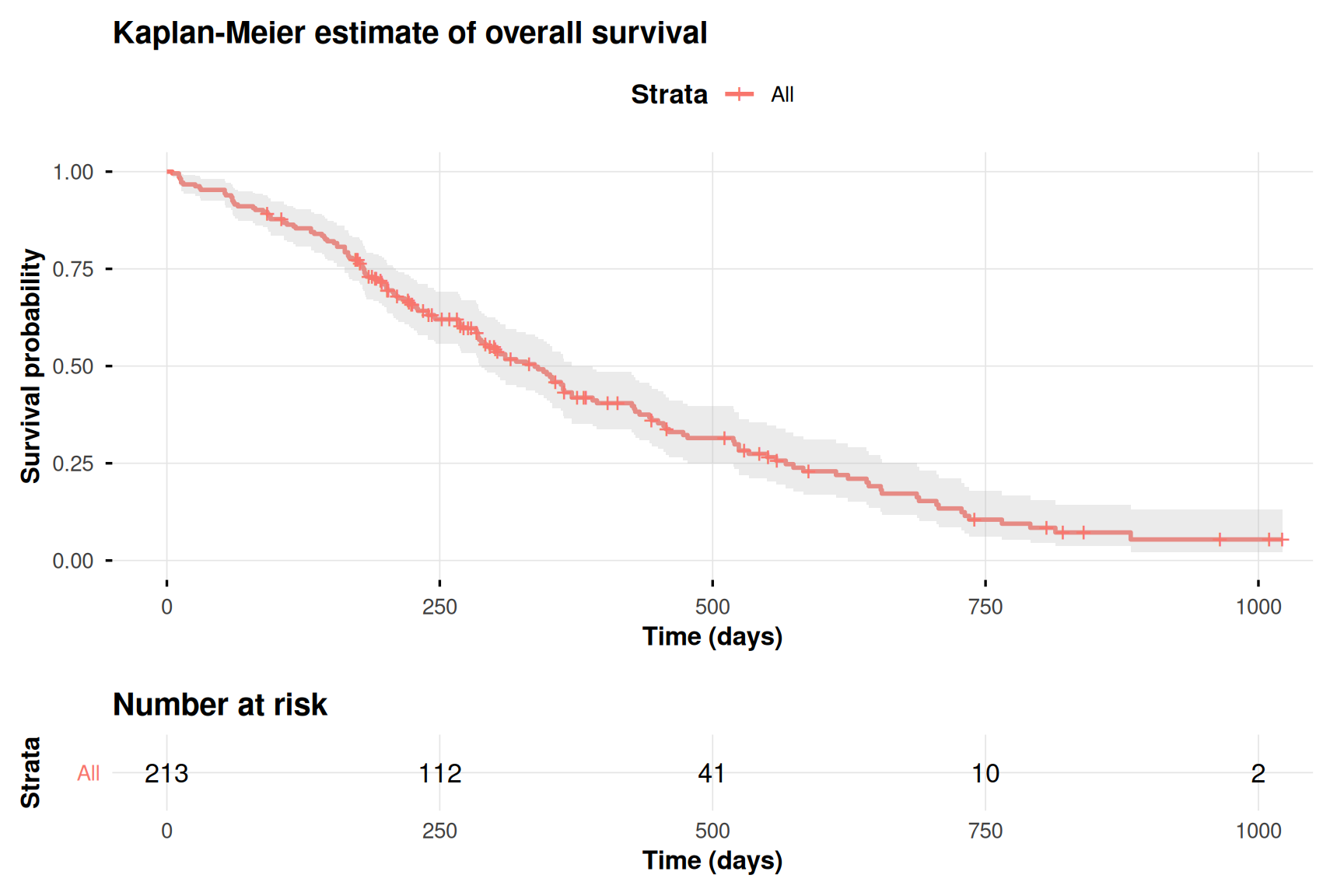
Censored individuals contribute to $n_j$ for as long as they are at risk, but never generate a $d_j$: this is precisely how the estimator uses the partial information they carry without assuming anything about their unobserved event time.
The variance of $\hat{S}(t)$ is estimated by **Greenwood's formula**, which is used to build the pointwise confidence bands shown around Kaplan-Meier curves below.
::: {.callout-note collapse="true" title="Greenwood's formula"}
$$
\widehat{\text{Var}}\big[\hat{S}(t)\big] = \hat{S}(t)^2 \sum_{j : t_{(j)} \leq t} \frac{d_j}{n_j (n_j - d_j)}
$$
:::
### Comparing two survival curves: the log-rank test
To test $H_0: S_1(t) = S_2(t)\ \forall t$ between two groups, the **log-rank test** compares, at each distinct event time $t_{(j)}$, the observed number of events in each group to the number that would be *expected* under $H_0$ (computed from a $2\times 2$ table of at-risk/event counts, in the same spirit as a Mantel-Haenszel test). Summing over all event times gives a test statistic that is asymptotically $\chi^2$-distributed under $H_0$:
$$
\chi^2 = \frac{\left(\sum_j (O_{1j} - E_{1j})\right)^2}{\sum_j V_j} \ \sim\ \chi^2_{(1)} \text{ under } H_0
$$
where $O_{1j}$, $E_{1j}$ and $V_j$ are respectively the observed events, expected events and variance in group 1 at $t_{(j)}$. The log-rank test is non-parametric and weights all event times equally; it is the standard tool to compare Kaplan-Meier curves visually and formally.
## Application: Kaplan-Meier estimation
::: panel-tabset
### Overall survival
```{r}
km_overall <- survfit(Surv(time, status) ~ 1, data = lung_cc)
km_overall
```
```{r, fig.width=9, fig.height=6}
ggsurvplot(
  km_overall,
  data = lung_cc,
  conf.int = TRUE,
  risk.table = TRUE,
  xlab = "Time (days)",
  ylab = "Survival probability",
  title = "Kaplan-Meier estimate of overall survival",
  palette = "viridis",
  ggtheme = theme_survival()
)
```
::: {.callout-tip title="Reading the curve"}
The median survival time (the time at which $\hat{S}(t) = 0.5$) and its confidence interval are read directly from the `survfit` summary above: `r summary(km_overall)$table["median"]` days, 95% CI \[`r summary(km_overall)$table["0.95LCL"]` ; `r summary(km_overall)$table["0.95UCL"]`\]. In other words, half of the patients in the sample are still alive beyond this point.
:::
### Survival by sex
```{r}
km_sex <- survfit(Surv(time, status) ~ sex, data = lung_cc)
km_sex
survdiff_sex <- survdiff(Surv(time, status) ~ sex, data = lung_cc)
survdiff_sex
```
```{r, fig.width=9, fig.height=6}
ggsurvplot(
  km_sex,
  data = lung_cc,
  conf.int = TRUE,
  pval = TRUE,
  risk.table = TRUE,
  xlab = "Time (days)",
  ylab = "Survival probability",
  legend.title = "Sex",
  title = "Kaplan-Meier estimate by sex",
  subtitle = "With log-rank test p-value",
  palette = "viridis",
  ggtheme = theme_survival()
)
```
::: {.callout-tip title="Reading the curve"}
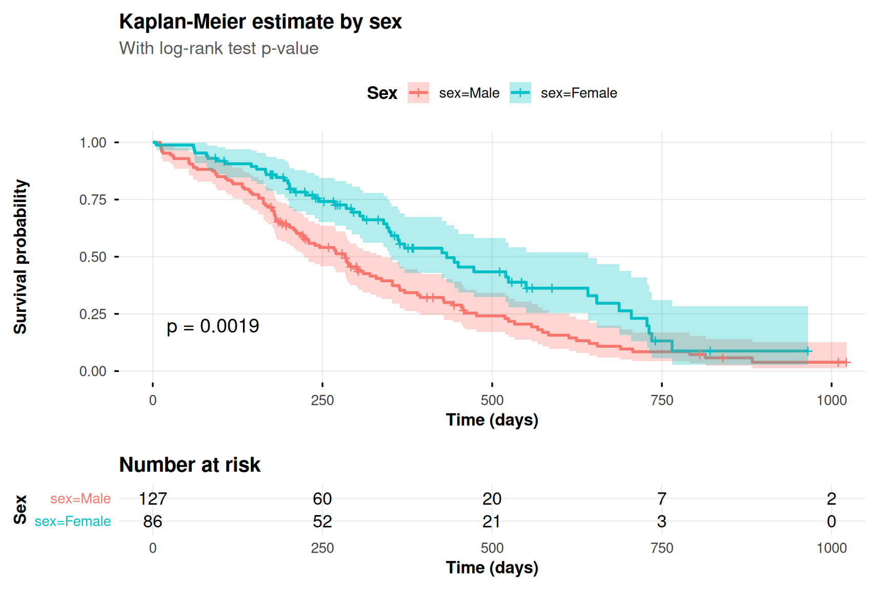
The log-rank test compares the two curves formally; the p-value displayed on the plot corresponds to the $\chi^2$ statistic described above. A separation between the curves that persists over the whole follow-up period, together with a small p-value, supports a genuine difference in survival between the two groups.
:::
### Survival by ECOG performance status
```{r}
km_ecog <- survfit(Surv(time, status) ~ ph.ecog_grouped, data = lung_cc)
```
```{r, fig.width=9, fig.height=6}
ggsurvplot(
  km_ecog,
  data = lung_cc,
  conf.int = FALSE,
  pval = TRUE,
  xlab = "Time (days)",
  ylab = "Survival probability",
  legend.title = "ECOG score",
  title = "Kaplan-Meier estimate by ECOG performance status",
  palette = "viridis",
  ggtheme = theme_survival()
)
```
::: {.callout-tip title="Reading the curve"}
As expected clinically, a higher ECOG score (worse functional status) is associated with a visibly lower survival curve. This descriptive result motivates including ECOG performance status in a multivariate model, to check whether its effect remains once other covariates are accounted for.
:::
:::
## The Cox proportional hazards model
### Theory
Kaplan-Meier curves and the log-rank test are well suited to compare a small number of groups, but they do not directly handle **several covariates at once**, nor **continuous** predictors such as age. The Cox proportional hazards model [@cox1972regression] fills this gap by modeling the hazard function as a baseline hazard modulated multiplicatively by covariates:
$$
h(t \mid X) = h_0(t) \exp\big(\beta^\top X\big) = h_0(t) \exp\left(\sum_{p=1}^{P} \beta_p X_p\right)
$$
where $h_0(t)$ is an unspecified **baseline hazard** (the hazard for an individual with $X = 0$), and $X = (X_1, \dots, X_P)$ is the covariate vector. The model is called **semi-parametric**: the covariate effects $\beta$ are estimated without ever specifying the functional form of $h_0(t)$.
**Proportional hazards assumption.** For two individuals with covariate vectors $X_a$ and $X_b$, the ratio of their hazards is constant over time:
$$
\frac{h(t \mid X_a)}{h(t \mid X_b)} = \frac{h_0(t)\exp(\beta^\top X_a)}{h_0(t)\exp(\beta^\top X_b)} = \exp\big(\beta^\top (X_a - X_b)\big)
$$
which does not depend on $t$ — hence the name of the model. In particular, for a one-unit increase in $X_p$ (all else held fixed), the hazard is multiplied by $\exp(\beta_p)$, the **hazard ratio (HR)** of covariate $p$:
$$
\text{HR}_p = \exp(\beta_p) = \frac{h(t \mid X_p + 1, X_{-p})}{h(t \mid X_p, X_{-p})}
$$
$\text{HR}_p > 1$ indicates an increased risk, $\text{HR}_p < 1$ a protective effect, and $\text{HR}_p = 1$ no effect.
**Estimation by partial likelihood.** Because $h_0(t)$ is left unspecified, $\beta$ cannot be estimated by ordinary maximum likelihood on the full hazard. Cox's key idea is to use only the *ordering* of event times, which leads to the following **partial likelihood**:
$$
L(\beta) = \prod_{j=1}^{k} \frac{\exp(\beta^\top X_{i(j)})}{\displaystyle\sum_{l \in R(t_{(j)})} \exp(\beta^\top X_l)}
$$
where $t_{(1)} < \dots < t_{(k)}$ are the distinct event times, $R(t_{(j)})$ is the **risk set** at $t_{(j)}$ (individuals still at risk just before $t_{(j)}$), and $i(j)$ is the individual who experiences the event at $t_{(j)}$. $\hat{\beta}$ is obtained by maximizing $\log L(\beta)$ numerically (Newton-Raphson), and standard errors follow from the curvature of the log-partial-likelihood at $\hat{\beta}$.
::: {.callout-note collapse="true" title="Detail: derivation of the partial likelihood"}
Conditional on an event occurring at $t_{(j)}$, the probability that it is individual $i \in R(t_{(j)})$ (rather than any other member of the risk set) who experiences it is:
$$
P\big(i \text{ fails at } t_{(j)} \mid \text{one failure in } R(t_{(j)})\big) = \frac{h_0(t_{(j)})\exp(\beta^\top X_i)}{\sum_{l \in R(t_{(j)})} h_0(t_{(j)})\exp(\beta^\top X_l)} = \frac{\exp(\beta^\top X_i)}{\sum_{l \in R(t_{(j)})} \exp(\beta^\top X_l)}
$$
Note that $h_0(t_{(j)})$ **cancels out** — this is precisely what allows $\beta$ to be estimated without ever modeling the baseline hazard. Multiplying these conditional probabilities over all observed event times gives the partial likelihood $L(\beta)$ stated above.
:::
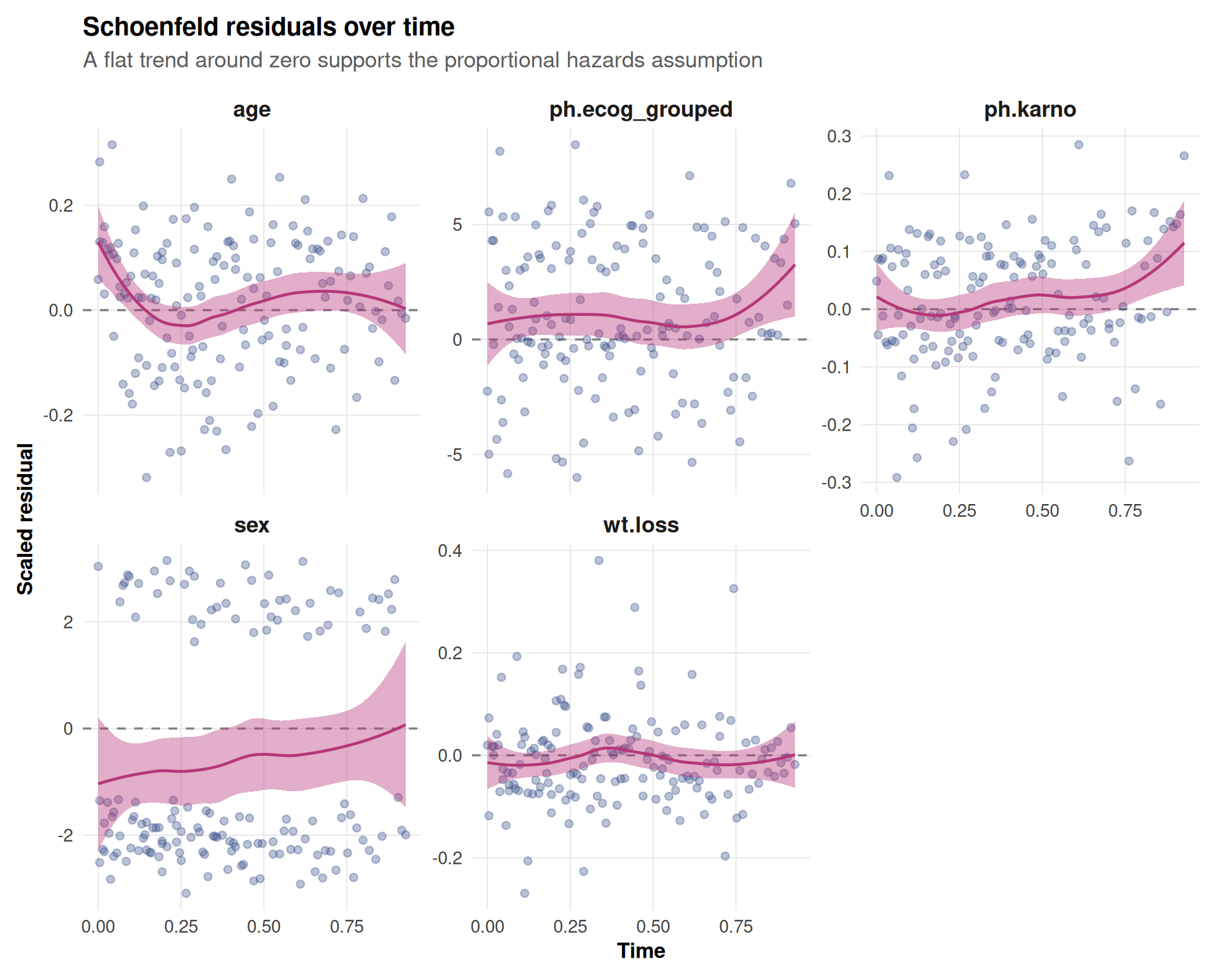
**Checking the assumption.** The proportional hazards assumption can be checked using **Schoenfeld residuals**: under $H_0$ (proportional hazards holds), these residuals should show no trend over time for each covariate. This is implemented in `R` by `cox.zph()`, illustrated below.
### Application: univariate and multivariate Cox models
::: panel-tabset
#### Univariate model (sex)
```{r}
cox_sex <- coxph(Surv(time, status) ~ sex, data = lung_cc)
summary(cox_sex)
```
```{r}
cox_table(cox_sex, caption = "Table 3: Hazard ratio for sex (univariate Cox model)")
```
::: {.callout-tip title="Interpretation"}
Being female (relative to male, the reference level) is associated with a hazard ratio below 1, i.e. a **lower** instantaneous risk of death, consistently with the Kaplan-Meier curves above.
:::
#### Multivariate model
```{r}
cox_multi <- coxph(
  Surv(time, status) ~ age + sex + ph.ecog_grouped + ph.karno + wt.loss,
  data = lung_cc
)
summary(cox_multi)
```
```{r}
cox_table(cox_multi, caption = "Table 4: Hazard ratios, multivariate Cox model")
```
```{r, fig.width=9, fig.height=6}
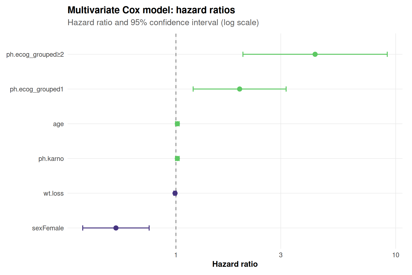
plot_forest(cox_multi, title = "Multivariate Cox model: hazard ratios")
```
::: {.callout-tip title="Reading the forest plot"}
Each point is the hazard ratio for one covariate, with its 95% confidence interval, on a log scale. Covariates whose interval excludes the dashed line at HR = 1 are significantly associated with survival, after adjusting for every other covariate in the model. Thanks to the regrouping performed earlier, `ph.ecog_grouped` now contributes stable, interpretable hazard ratios instead of the single-patient artifact seen on the raw four-level factor.
:::
:::
### Checking the proportional hazards assumption
```{r}
ph_test <- cox.zph(cox_multi)
ph_test
```
```{r, fig.width=10, fig.height=8}
plot_schoenfeld(ph_test)
```
::: {.callout-important title="How to read this diagnostic"}
A non-significant p-value for a given covariate (and for the global test) supports the proportional hazards assumption for that covariate. A significant p-value, or a Schoenfeld residual plot showing a clear trend over time rather than a flat scatter around zero, signals a violation that may require a time-varying coefficient, stratification, or an alternative model.
Even when the **global test** is not significant, always check each individual row: it is common for one covariate — `ph.karno` is a frequent candidate in this dataset — to show a nominally significant departure from proportionality on its own. This does not invalidate the model overall, but the hazard ratio for that covariate should then be interpreted as an *average effect over the follow-up period* rather than a strictly constant one.
:::
## Model selection
::: panel-tabset
### Nested model comparison
The univariate model (`cox_sex`) is nested within the multivariate model (`cox_multi`) once restricted to their common variables; more directly, we can compare the multivariate model to a reduced model to test whether a given covariate improves the fit, using a **likelihood ratio test**:
```{r}
cox_reduced <- coxph(Surv(time, status) ~ age + sex + ph.karno + wt.loss, data = lung_cc)

anova(cox_reduced, cox_multi)
```
::: {.callout-tip title="Interpretation"}
A significant p-value indicates that adding `ph.ecog_grouped` significantly improves the fit relative to the reduced model.
:::
### Concordance and AIC
```{r}
tibble::tibble(
  Model = c("Univariate (sex)", "Reduced (no ph.ecog)", "Multivariate"),
  AIC = c(AIC(cox_sex), AIC(cox_reduced), AIC(cox_multi)),
  Concordance = c(
    summary(cox_sex)$concordance[1],
    summary(cox_reduced)$concordance[1],
    summary(cox_multi)$concordance[1]
  )
) %>%
  mutate(across(where(is.numeric), ~ round(.x, 3))) %>%
  kable(caption = "Table 5: Model comparison, AIC and concordance index")
```
::: {.callout-tip title="Interpretation"}
The **concordance index** (C-index) generalizes the AUC to survival data: it estimates the probability that, for a randomly chosen pair of individuals, the one predicted to have the higher risk indeed experiences the event first. Together with AIC (lower is better) and the likelihood ratio test above, it supports retaining the multivariate model including `ph.ecog_grouped`.
:::
:::
## Beyond the Cox model
The Cox model covers the large majority of applied survival analyses, but the field extends further in several directions that are worth knowing about even without full development here:
::: {.callout-note collapse="true" title="Parametric, frailty and competing risks models"}
- **Parametric models** (e.g. Weibull, log-logistic Accelerated Failure Time models, fitted with `survreg()` or `flexsurv::flexsurvreg()`) specify a full distribution for $T$, which allows extrapolation beyond the observed follow-up — something the semi-parametric Cox model cannot do, since $h_0(t)$ is never estimated outside the observed event times.
- **Frailty models** add a random effect (frailty term) to the hazard to account for unobserved heterogeneity or clustering (e.g. repeated measures, family/hospital clustering).
- **Competing risks models** (e.g. Fine-Gray subdistribution hazards) are needed when individuals can experience one of several mutually exclusive event types (e.g. death from disease vs. death from other causes), since standard Kaplan-Meier curves overestimate the cumulative incidence of a specific cause in that setting.
:::
## Results
Across the descriptive, Kaplan-Meier and Cox analyses of the `lung` dataset, sex and functional status (ECOG, Karnofsky) emerge as the covariates most consistently associated with survival, while the proportional hazards assumption is reasonably well supported overall for the retained model, modulo the per-covariate caveat discussed above (see `cox.zph` output above). Substantively, this replicates a well documented pattern in this benchmark dataset: **female patients and patients with better performance status have a lower hazard of death**, i.e. a better prognosis, after adjusting for age and weight loss.
A methodological point worth remembering for future analyses: the ECOG level `3` was reduced to a single patient once missing values were dropped. Rather than discarding that observation, grouping it with the neighboring `2` level kept the information while avoiding a hazard ratio estimated from one person — a pattern to watch for whenever a categorical covariate has a sparse level.
Methodologically, this tutorial illustrates the general survival-analysis workflow: (1) characterize censoring and follow-up, (2) use Kaplan-Meier and the log-rank test for a first, assumption-light description, (3) move to the Cox model to adjust for several covariates simultaneously, and (4) always check the proportional hazards assumption before trusting the hazard ratios.
::: {.callout-tip title="Key takeaways"}
- Always characterize the censoring pattern before any modeling — censoring is partial information, not missing data.
- Use Kaplan-Meier and the log-rank test for a first, assumption-light look at survival, one or two groups at a time.
- Move to the Cox model to adjust for several covariates simultaneously; $\exp(\beta_p)$ is read as a hazard ratio.
- Never trust hazard ratios without checking the proportional hazards assumption (`cox.zph()`, Schoenfeld residuals).
:::
## Computational informations
<details>
<summary>Session informations</summary>
```{r session_info, results='markup'}
devtools::session_info()
```
</details>