---
title: "Differential Proteomics Analysis with DESeq2: From Spectral Counts to Biological Interpretation"
author: "Clément Poupelin"
date: 07-16-2026
date-modified: "`r Sys.Date()`"
bibliography: references.bib
format:
html:
embed-resources: false
toc: true
code-fold: true
code-summary: "Show the code"
code-tools: true
toc-location: right
page-layout: article
code-overflow: wrap
number-sections: false
editor: visual
categories: ["Proteomics", "DESeq2", "Bioinformatics"]
description: "A pedagogical introduction to differential proteomics analysis with DESeq2: state of the art, mathematical theory of the negative binomial model, and a full R application on a real spike-in benchmark dataset."
execute:
echo: true
warning: false
message: false
error: true
---
## Setup
::: panel-tabset
### packages
```{r}
library(dplyr)        ## Data manipulation
library(tidyr)        ## Data manipulation
library(tibble)        ## Data manipulation
library(ggplot2)       ## Plots
library(ggrepel)       ## Non-overlapping labels on volcano plots
library(viridis)       ## Colorblind palette
library(pheatmap)      ## Heatmaps

library(DESeq2)        ## Differential analysis of count data
library(apeglm)        ## Shrinkage of log2 fold changes
library(vsn)            ## Variance stabilizing transformation diagnostics

## Note: no proteomics-specific data package (e.g. DAPARdata/MSnbase) is
## needed. The tutorial dataset is simulated directly below (see the
## "Choice of Dataset" section), so DESeq2 is used exactly as it would be
## on any already-exported count matrix, real or simulated.


library(broom)          ## Tidy model outputs
library(knitr)          ## Tables
library(kableExtra)     ## Table styling
library(DT)              ## Interactive tables
```
### Functions
```{r}
## Consistent ggplot2 theme used across every figure in the report, for a
## clean, "modern research article" look, matching the style used in the
## survival-analysis and SEM companion reports.
theme_proteo <- function(base_size = 13) {
  theme_minimal(base_size = base_size, base_family = "sans") +
    theme(
      plot.title = element_text(face = "bold", size = rel(1.15), margin = margin(b = 6)),
      plot.subtitle = element_text(color = "grey35", margin = margin(b = 10)),
      axis.title = element_text(face = "bold", size = rel(0.95)),
      axis.text = element_text(color = "grey25"),
      panel.grid.minor = element_blank(),
      panel.grid.major = element_line(color = "grey90", linewidth = 0.3),
      legend.position = "top",
      legend.title = element_text(face = "bold"),
      strip.text = element_text(face = "bold", size = rel(1)),
      plot.margin = margin(10, 15, 10, 10)
    )
}

## Volcano plot from a DESeq2 results data.frame (as produced by
## as.data.frame(results(dds))), with viridis coloring of significant hits
## and automatic labeling of the top proteins.
plot_volcano <- function(res_df, lfc_thresh = 1, alpha = 0.05,
                          title = "Volcano plot", n_labels = 10) {
  res_df <- res_df %>%
    mutate(
      protein = rownames(.),
      status = case_when(
        padj < alpha & log2FoldChange >  lfc_thresh ~ "Up",
        padj < alpha & log2FoldChange < -lfc_thresh ~ "Down",
        TRUE ~ "NS"
      )
    )

  top_hits <- res_df %>%
    filter(status != "NS") %>%
    arrange(padj) %>%
    slice_head(n = n_labels)

  ggplot(res_df, aes(x = log2FoldChange, y = -log10(padj), color = status)) +
    geom_point(alpha = 0.65, size = 1.8) +
    geom_vline(xintercept = c(-lfc_thresh, lfc_thresh), linetype = "dashed", color = "grey50") +
    geom_hline(yintercept = -log10(alpha), linetype = "dashed", color = "grey50") +
    ggrepel::geom_text_repel(data = top_hits, aes(label = protein),
                              size = 3, color = "grey15", max.overlaps = 20,
                              segment.size = 0.3) +
    scale_color_manual(values = c(Up = "#B63679", Down = "#21918C", NS = "grey70")) +
    labs(title = title, x = expression(log[2]~"fold change"),
         y = expression(-log[10]~"adjusted p-value"), color = NULL) +
    theme_proteo()
}

## MA plot (mean normalized count vs. log2 fold change), rebuilt in ggplot2
## from a DESeq2 results table for a research-article look.
plot_ma <- function(res_df, lfc_thresh = 1, alpha = 0.05, title = "MA plot") {
  res_df <- res_df %>%
    mutate(
      protein = rownames(.),
      status = case_when(
        padj < alpha & log2FoldChange >  lfc_thresh ~ "Up",
        padj < alpha & log2FoldChange < -lfc_thresh ~ "Down",
        TRUE ~ "NS"
      )
    ) %>%
    filter(!is.na(padj))

  ggplot(res_df, aes(x = baseMean, y = log2FoldChange, color = status)) +
    geom_point(alpha = 0.65, size = 1.8) +
    geom_hline(yintercept = 0, color = "grey40", linewidth = 0.4) +
    scale_x_log10() +
    scale_color_manual(values = c(Up = "#B63679", Down = "#21918C", NS = "grey70")) +
    labs(title = title, x = "Mean of normalized counts", y = expression(log[2]~"fold change"),
         color = NULL) +
    theme_proteo()
}

## PCA plot from a variance-stabilized DESeqTransform object.
plot_pca_proteo <- function(vsd, intgroup = "condition", title = "PCA of samples") {
  pca_data <- DESeq2::plotPCA(vsd, intgroup = intgroup, returnData = TRUE)
  percent_var <- round(100 * attr(pca_data, "percentVar"))

  ggplot(pca_data, aes(x = PC1, y = PC2, color = .data[[intgroup]], label = name)) +
    geom_point(size = 3.2, alpha = 0.85) +
    ggrepel::geom_text_repel(size = 3, color = "grey20", max.overlaps = 20) +
    scale_color_viridis_d(option = "D", end = 0.85) +
    labs(title = title, x = paste0("PC1 (", percent_var[1], "% variance)"),
         y = paste0("PC2 (", percent_var[2], "% variance)"), color = "Condition") +
    theme_proteo()
}

## Dispersion plot rebuilt in ggplot2 from a DESeqDataSet, mirroring
## DESeq2::plotDispEsts() but in the report's visual style.
plot_dispersions <- function(dds, title = "Dispersion estimates") {
  tibble(
    baseMean = mcols(dds)$baseMean,
    gene_est = mcols(dds)$dispGeneEst,
    fitted   = mcols(dds)$dispFit,
    final    = mcols(dds)$dispersion
  ) %>%
    filter(baseMean > 0) %>%
    pivot_longer(cols = c(gene_est, fitted, final), names_to = "type", values_to = "dispersion") %>%
    mutate(type = recode(type,
                          gene_est = "Gene-wise estimate",
                          fitted   = "Fitted trend",
                          final    = "Final (shrunk) estimate")) %>%
    ggplot(aes(x = baseMean, y = dispersion, color = type)) +
    geom_point(data = . %>% filter(type == "Gene-wise estimate"), alpha = 0.4, size = 1.2) +
    geom_point(data = . %>% filter(type == "Final (shrunk) estimate"), alpha = 0.6, size = 1.2) +
    geom_line(data = . %>% filter(type == "Fitted trend"), linewidth = 0.9) +
    scale_x_log10() + scale_y_log10() +
    scale_color_manual(values = c("Gene-wise estimate" = "grey60",
                                   "Fitted trend" = "#B63679",
                                   "Final (shrunk) estimate" = "#21918C")) +
    labs(title = title, x = "Mean of normalized counts", y = "Dispersion", color = NULL) +
    theme_proteo()
}

## Tidy DESeq2 results into a publication-ready table.
deseq_table <- function(res, caption = NULL, n = 15) {
  as.data.frame(res) %>%
    rownames_to_column("Protein") %>%
    arrange(padj) %>%
    slice_head(n = n) %>%
    transmute(
      Protein,
      baseMean = round(baseMean, 1),
      log2FC = round(log2FoldChange, 3),
      lfcSE = round(lfcSE, 3),
      stat = round(stat, 2),
      pvalue = signif(pvalue, 3),
      padj = signif(padj, 3)
    ) %>%
    kable(caption = caption) %>%
    kable_styling(full_width = FALSE)
}
```
### Seed
```{r}
set.seed(140400)
```
:::
## Abstract
This tutorial provides a self-contained, pedagogical introduction to **differential proteomics analysis with `DESeq2`**, the negative-binomial count model originally designed for RNA-seq [@love2014moderated] and now routinely repurposed for mass-spectrometry-based proteomics count data [@anders2010differential].\
It follows the same structure as the companion reports on [Structural Equation Modeling](http://clement-poupelin.github.io/publications.html) and on [Survival Analysis](http://clement-poupelin.github.io/publications.html): a state-of-the-art review, the underlying mathematical theory, and a complete, reproducible `R` application — here on a spike-in proteomics design with a known ground truth, reproducing the real published benchmark of Ramus et al. (2016) [@ramus2016spiked] with calibrated, well-behaved simulated counts so that the standard `DESeq2` workflow can be walked through exactly as documented (see the [dataset section](#dataset) for the rationale, and the callouts throughout for what changes on rougher, real exported data).
The goal is to give researchers and students a rigorous but accessible entry point into count-based differential proteomics: what DESeq2 assumes, why these assumptions are only partially met by proteomics data, and how to run, diagnose and interpret the analysis in practice.
## State of the Art: DESeq2 Applied to Proteomics
### From transcriptomics to proteomics: why the transfer is tempting
`DESeq2` was designed to detect **differentially expressed genes** from RNA-seq **read counts**: for each gene $i$ and sample $j$, the raw number of sequencing reads mapped to that gene [@love2014moderated; @anders2010differential]. Formally, this is a matrix of non-negative integers, one row per gene, one column per sample — exactly the kind of object that also arises naturally in several other high-throughput count-based assays: ChIP-seq, Hi-C, shRNA screens, and — importantly here — **mass-spectrometry-based proteomics**, where the "count" for a protein can be the number of **peptide-spectrum matches (PSMs)** or **spectral counts** assigned to it in a given sample <cite index="4-1,5-1">the value in the i-th row and the j-th column of such matrices can correspond to peptide sequences quantified by mass spectrometry, just as it corresponds to genes in RNA-seq</cite>.
This structural analogy — a matrix of counts, biological replicates, one or more experimental factors — is what motivates using DESeq2 (or its sibling `edgeR`) directly on proteomics spectral-count data, an approach explored since the early 2010s <cite index="10-1">under the name "MultiSpec", applying RNA-seq differential-expression tools (edgeR, DESeq and baySeq) to label-free spectral-count proteomics data by analogy with RNA sequencing</cite>.
::: {.callout-note collapse="true" title="Reminder: what exactly is a spectral count?"}
In shotgun (bottom-up) proteomics, proteins are digested into peptides which are then measured by tandem mass spectrometry (LC-MS/MS). Each time a peptide triggers a fragmentation spectrum that is confidently matched to a sequence, this produces one **peptide-spectrum match (PSM)**. Summing the number of PSMs assigned to all peptides of a given protein, in a given sample, yields the **spectral count** of that protein — a non-negative integer, directly analogous to a gene's read count in RNA-seq. This is different from (and computed upstream of) continuous, transformed quantities such as **LFQ intensities** or **iBAQ values**, which are the other major family of proteomics quantification and are *not* count data.
:::
### The negative binomial model and its statistical assumptions
DESeq2 models the counts $K_{ij}$ (gene/protein $i$, sample $j$) as realizations of a **negative binomial (NB)** distribution:
$$
K_{ij} \sim \text{NB}\big(\mu_{ij}, \alpha_i\big), \qquad \mu_{ij} = s_j \, q_{ij}
$$
where $s_j$ is a sample-specific **size factor** (normalization) and $q_{ij}$ reflects the true relative abundance of feature $i$ in the condition of sample $j$; $\alpha_i$ is a **feature-specific dispersion** parameter that captures biological variability beyond Poisson (shot-noise) variance. The full theoretical development is given in the [dedicated theory section](#theory) below. The key assumptions this places on the data are:
- **Discreteness**: the input must be raw, un-normalized, non-negative integer counts — not intensities, ratios, or already-normalized values <cite index="4-1">this is important for DESeq2's statistical model to hold, as only the actual counts allow assessing the measurement precision correctly</cite>.
- **Mean-variance relationship**: the variance of each feature across replicates is expected to grow with its mean, following the NB law $\text{Var}(K_{ij}) = \mu_{ij} + \alpha_i \mu_{ij}^2$ — this needs to be checked, not assumed.
- **A moderate number of features with true zero effect**, used by DESeq2's normalization and independent filtering procedures; and **enough replicates** (ideally $\geq 3$ per condition) for dispersion estimation to be reliable.
### Adaptations, empirical evidence and limits specific to proteomics
Applying an RNA-seq-born model to proteomics count data is statistically legitimate in principle, but several proteomics-specific features complicate the picture:
::: {.callout-important title="Points of methodological vigilance"}
- **Lower, noisier counts.** Spectral counts per protein are typically far smaller than RNA-seq read counts per gene (tens rather than thousands), and the Benjamini–Hochberg correction is often preferred over DESeq2/DESeq's own independent-filtering defaults precisely <cite index="6-1">because of the low count numbers in proteomics compared to RNA-seq</cite>.
- **Model fit is data-dependent, not guaranteed.** There is no theoretical obstruction to using DESeq2 on non-sequencing count data, but whether the negative-binomial error model actually fits a given proteomics dataset must be checked empirically (MA plots between replicates, residual diagnostics), rather than assumed by analogy with RNA-seq.
- **Missing values are structural, not random.** Unlike RNA-seq (where a true zero count is informative), proteomics data — especially continuous LFQ intensities — often contain **missing-not-at-random** values below the instrument's limit of detection. DESeq2 has no missing-value model; when spectral counts are used, genuine zeros are valid counts, but one must distinguish them from proteins that were never *searched for* in a given run.
- **Compressed dynamic range and technical drift.** Ratio compression, carry-over, and batch effects across MS runs can distort the fold changes recovered from count-based proteomics more than from RNA-seq.
- **PSM counts are compositional and length-biased**: longer proteins and proteins with more "flyable" (easily ionized) peptides accumulate more PSMs, independently of true abundance — a source of technical variance that DESeq2's per-feature dispersion partially, but not fully, absorbs.
:::
A direct comparative evaluation of differential-expression methods on real spiked proteomics data found that <cite index="6-1">QSpec and DESeq performed comparatively well across benchmark scenarios, and the study suggested performing future differential expression analyses with either QSpec or DESeq, or a combination of the two</cite>, while also cautioning that combining all seven benchmarked methods inflated the false-positive rate. This supports using DESeq2 as one credible tool in the proteomics toolbox — not a universally superior one — and motivates the shrinkage/FDR safeguards detailed in the [theory section](#theory).
Because of these differences, dedicated proteomics-specific alternatives (`limma`, `MSstats`, `DEP`, `DEqMS`) have also been developed; `DEqMS` in particular directly targets the variance-estimation issue by <cite index="7-1">modelling the hierarchical PSM → peptide → protein data structure of shotgun mass spectrometry proteomics data explicitly</cite>, rather than treating protein-level counts as an undifferentiated matrix. DESeq2 remains, however, a well-documented, actively maintained and pedagogically transparent entry point — which is why it is the focus of this tutorial.
## Resources for Further Reading {#resources}
The following resources — freely available online — were used to build this report and are recommended for anyone who wants to go deeper.
::: panel-tabset
### Official tutorials & documentation
- **[DESeq2 Bioconductor vignette](https://bioconductor.org/packages/release/bioc/vignettes/DESeq2/inst/doc/DESeq2.html)** — the canonical reference for every function used in this report (`DESeqDataSetFromMatrix`, `DESeq()`, `results()`, `lfcShrink()`, `plotPCA()`, `plotDispEsts()`...), including the statistical background and worked examples.
- **[RNA-seq workflow: gene-level exploratory analysis and differential expression (Bioconductor)](https://bioconductor.org/packages/release/workflows/vignettes/rnaseqGene/inst/doc/rnaseqGene.html)** — a slower-paced companion to the vignette above, covering count-matrix construction from scratch; useful to understand where the "counts" actually come from before adapting the workflow to proteomics.
- **[USDA-ARS SEAStats — Demo 4: Differential expression with DESeq2](https://usda-ree-ars.github.io/SEAStats/multiomics_demo/Demo4_DESeq2.html)** — a concise, modified version of the official vignette explicitly framed for a multi-omics audience, useful as a quick refresher on the standard `R` workflow.
- **[Bioconductor Support forum: "Protein differential Expression analysis"](https://support.bioconductor.org/p/104642/)** — a thread by DESeq2's own maintainers discussing, in their words, exactly why and under which conditions DESeq2 can (or cannot) be trusted on proteomics count data. Essential reading before applying the method blindly.
### Reference research articles
- **Love, Huber & Anders (2014), *Moderated estimation of fold change and dispersion for RNA-seq data with DESeq2*, Genome Biology** [@love2014moderated] — the DESeq2 method paper itself; open access at the [publisher's site](https://genomebiology.biomedcentral.com/articles/10.1186/s13059-014-0550-8). Source of the mathematical model developed in this report.
- **Anders & Huber (2010), *Differential expression analysis for sequence count data*, Genome Biology** [@anders2010differential] — the original DESeq paper introducing the median-of-ratios normalization and NB modeling framework that DESeq2 builds on.
- **Zhu, Ibrahim & Love (2019), *Heavy-tailed prior distributions for sequence count data: removing the noise and preserving large differences***, Bioinformatics — introduces `apeglm`, the adaptive shrinkage estimator for log2 fold changes used in this report's `lfcShrink()` calls.
- **Langley & Mayr (2015), *Comparative analysis of statistical methods used for detecting differential expression in label-free mass spectrometry proteomics*, Journal of Proteomics** [@langley2015comparative] — a rigorous benchmark of DESeq/DESeq2, edgeR, limma, QSpec and others directly on proteomics spike-in data; the main empirical source for the "points of methodological vigilance" discussed above.
- **Vega Yu et al. (2020), *DEqMS: a method for accurate variance estimation in differential protein expression analysis*, Molecular & Cellular Proteomics** [@vega2020deqms] — a proteomics-native alternative to DESeq2/limma, useful for contextualizing this report's method relative to the state of the art.
- **Ramus et al. (2016), *Spiked proteomic standard dataset for testing label-free quantitative software and statistical methods*, Data in Brief / Journal of Proteomics** [@ramus2016spiked] — describes the ground-truth benchmark dataset used for the application in this report (see next section).
### Community tutorials
- **[Prostar / DAPAR project documentation](https://prostar-proteomics.github.io/)** — the Bioconductor ecosystem (`DAPAR`, `DAPARdata`) that distributes the Ramus et al. dataset used here in an analysis-ready `R` format, together with tutorials on proteomics-specific preprocessing (missing-value handling, normalization, aggregation).
- **[ProFI Proteomics — "Details of the Yeast-UPS1 spiked-in experiment"](https://www.profiproteomics.fr/details-of-the-profi-yeast-ups1-spiked-in-experiment/)** — background and raw-data access for the PXD001819 dataset used in this tutorial.
- **[GTPB IBIP19 course — "Quality control of label-free quantification MS data"](https://gtpb.github.io/IBIP19/pages/qc/yeast-ups1)** — a hands-on bioinformatics course module that uses the same Ramus et al. yeast/UPS1 dataset for teaching proteomics QC, complementary to the differential-analysis focus of this report.
:::
## Choice of Dataset: a Yeast / UPS1 Spike-in Design {#dataset}
### Why this design, and a practical note on the data used below
Pedagogically, differential analysis is only fully convincing when the **ground truth is known**, so that the method's sensitivity and false-discovery behavior can actually be checked rather than merely trusted. This rules out most "real" biological datasets, where nobody truly knows which proteins are differential. The design retained here reproduces the **spike-in benchmark of Ramus et al. (2016)** [@ramus2016spiked], among the most widely used ground-truth designs in the quantitative proteomics literature, deposited under **PXD001819** on the [PRIDE / ProteomeXchange](https://www.ebi.ac.uk/pride/) repository:
::: {.callout-tip title="Design of the Ramus et al. benchmark"}
A **constant background** of yeast (*Saccharomyces cerevisiae*) whole-cell lysate is spiked with an **equimolar mixture of 48 human recombinant proteins (Sigma UPS1)**, at two different concentrations, each condition analyzed in **triplicate** by nanoLC-MS/MS. Because the yeast background is strictly constant across samples while the UPS1 proteins vary by design, the **48 UPS1 proteins constitute the known "true positives"**, and the yeast background proteins constitute the known "true negatives" for any pairwise comparison between two spike-in levels — allowing an actual sensitivity/specificity check of the DESeq2 workflow, rather than only a list of hits with no way to verify them.
:::
::: {.callout-important title="Why this tutorial uses calibrated simulated counts rather than the raw PXD001819 export"}
For a **first, standard-case tutorial**, the priority is that the classic `DESeq2` functions (`DESeq()`, `vst()`, `lfcShrink()`...) run exactly as documented, with no detour. Reprocessing the raw PXD001819 files end-to-end would require a full search-engine pipeline (Mascot/MaxQuant) to obtain genuine peptide-spectrum-match counts — out of scope here — and the readily distributable text export of this dataset only exposes continuous **intensities**, not native spectral counts; turning it into counts via a coarse proxy (as a first version of this report did) compresses the dynamic range enough to break DESeq2's default dispersion-trend fitting and `vst()`'s subsampling heuristic (see the callouts further below for exactly why).
We therefore **simulate a count matrix**, calibrated to realistic spectral-count magnitudes and negative-binomial dispersions reported in the proteomics literature, but reproducing **exactly the real experimental design** of Ramus et al. (2016): a constant yeast background, 48 spiked human UPS1 proteins with a known, realistic fold change between two spike-in levels, and 3 replicates per condition. This keeps the ground truth exact and the workflow textbook-standard, which is the right starting point before tackling the rougher edges of real exported data (briefly discussed at the end of this report). Swapping in a genuine PSM-count export from a reprocessed PXD001819 search (or any other real study) requires no change beyond the [import code](#dataset) below.
:::
### Simulating the count matrix
```{r}
n_yeast <- 2000    ## constant background proteins ("true negatives")
n_ups1  <- 48      ## spiked human UPS1 proteins ("true positives")
n_rep   <- 3        ## replicates per condition, as in Ramus et al. (2016)

col_data <- data.frame(
  condition = factor(rep(c("Low_spike", "High_spike"), each = n_rep),
                      levels = c("Low_spike", "High_spike")),
  row.names = paste0("sample", seq_len(2 * n_rep))
)

## Realistic per-protein mean spectral counts (log-normal across proteins,
## as typically observed) and negative-binomial dispersions decreasing
## with abundance -- both calibrated to typical shotgun-proteomics scales.
yeast_mean <- rlnorm(n_yeast, meanlog = log(30), sdlog = 1)
yeast_disp <- 0.15 + 0.3 * exp(-yeast_mean / 40)

ups1_mean_low <- rlnorm(n_ups1, meanlog = log(15), sdlog = 0.8)
true_log2fc   <- rep(2.5, n_ups1)                 ## known, designed spike-in effect
ups1_mean_high <- ups1_mean_low * 2^true_log2fc
ups1_disp <- 0.15 + 0.3 * exp(-ups1_mean_low / 40)

## Small, realistic per-sample depth variation (as between real MS runs).
depth_factor <- rlnorm(2 * n_rep, meanlog = 0, sdlog = 0.15)

protein_ids <- c(paste0("sp|YEAST", sprintf("%04d", seq_len(n_yeast)), "|BACKGROUND_YEAST"),
                  paste0("sp|UPS1_", sprintf("%02d", seq_len(n_ups1)), "|SPIKE_HUMAN"))

count_matrix <- matrix(0L, nrow = n_yeast + n_ups1, ncol = 2 * n_rep,
                        dimnames = list(protein_ids, rownames(col_data)))

for (j in seq_len(2 * n_rep)) {
  is_high <- col_data$condition[j] == "High_spike"
  mu_yeast <- yeast_mean * depth_factor[j]
  mu_ups1  <- (if (is_high) ups1_mean_high else ups1_mean_low) * depth_factor[j]

  count_matrix[seq_len(n_yeast), j] <- rnbinom(n_yeast, mu = mu_yeast, size = 1 / yeast_disp)
  count_matrix[n_yeast + seq_len(n_ups1), j] <- rnbinom(n_ups1, mu = mu_ups1, size = 1 / ups1_disp)
}
```
The resulting object is exactly the input `DESeq2` expects: **a matrix of non-negative integer counts, one row per protein, one column per sample**. This is the crucial structural point of this whole tutorial:
::: {.callout-important title="Expected shape of the data for DESeq2"}
- **Rows**: proteins (or protein groups), identified by a unique row name (protein/UniProt accession).
- **Columns**: samples (biological or technical replicates).
- **Values**: non-negative **integers** — raw spectral/PSM counts, never normalized values, never intensities, never log-transformed values.
- A separate **`colData`** data frame, with **one row per sample in the same order as the count matrix's columns**, describing the experimental factor(s) (here: spike-in concentration / condition).
- A **design formula**, e.g. `~ condition`, telling DESeq2 which column(s) of `colData` define the comparison of interest.
This is structurally identical to the RNA-seq case — only the biological meaning of a "count" changes.
:::
It includes `r nrow(count_matrix)` proteins characterized across `r ncol(count_matrix)` samples, distributed in `r nlevels(col_data$condition)` conditions (`r paste(levels(col_data$condition), collapse = " vs. ")`), each replicated `r n_rep` times.
```{r}
count_matrix %>%
  as.data.frame() %>%
  rownames_to_column("Protein") %>%
  DT::datatable()
```
::: {.callout-note collapse="true" title="What happens with rougher, real exported data (and how to recognize it)"}
Real proteomics exports are considerably messier than the clean simulation above, and it is worth knowing the typical symptoms in advance rather than discovering them mid-analysis:
- **Coarse or compressed counts.** When only continuous LFQ/MaxQuant intensities are available and a proxy count is derived from them (e.g. "number of quantified peptides per protein"), the resulting dynamic range is often too narrow for DESeq2's default **parametric** dispersion-trend fitting, which then raises an explicit error (*"all gene-wise dispersion estimates are within 2 orders of magnitude from the minimum value..."*) rather than silently returning an unreliable fit. DESeq2's own suggested remedy — retrying with `fitType = "local"`, or, as a last resort, using the raw gene-wise dispersion estimates as final — is the right response, but the deeper fix is to obtain finer-grained counts (genuine PSM/spectral counts) whenever possible.
- **`vst()` refusing to run.** `vst()` uses a fast heuristic that subsamples proteins with mean normalized count above 5 to fit its internal trend; with coarse or low-count proxies, too few proteins may clear that bar, and `vst()` will explicitly recommend calling `varianceStabilizingTransformation()` directly, or, as an even lighter fallback, using `normTransform()` (a simple log2(normalized count + 1) transform that needs no dispersion-trend fitting at all) for the exploratory PCA/heatmap plots.
- **Missing or duplicated protein identifiers.** Real search-engine exports routinely contain peptide/protein rows with a blank or `NA` group identifier (ambiguous matches, contaminants); aggregating to the protein level without first filtering these out produces a row with a missing name, which `R` refuses to use in a matrix (`as.matrix()` errors with *"missing values in 'row.names' are not allowed"*).
- **Heavy compiled dependencies.** Bioconductor packages built for reading raw MS files (e.g. `mzR`, pulled in transitively by `MSnbase`/`DAPARdata`) wrap external C/C++ libraries (netCDF, Boost) and are a frequent, platform-dependent source of installation failures unrelated to the statistics itself. When only an already-exported text table is needed, it is often simpler and more robust to read it directly (`read.table()`) than to install the full raw-data-reading stack.
None of these issues affect the clean, simulated dataset used in the rest of this tutorial — they are flagged here so they are recognized as normal, documented behavior if encountered on a real dataset, rather than mistaken for a bug in the code.
:::
### The negative binomial generalized linear model
For protein $i$ ($i = 1, \dots, n$) and sample $j$ ($j = 1, \dots, m$), let $K_{ij}$ denote the observed count. DESeq2 assumes:
$$
K_{ij} \sim \text{NB}(\mu_{ij}, \alpha_i)
$$
with mean and variance:
$$
\mathbb{E}[K_{ij}] = \mu_{ij} = s_j \, q_{ij}, \qquad \text{Var}(K_{ij}) = \mu_{ij} + \alpha_i \, \mu_{ij}^2
$$
The variance is decomposed into a **Poisson (shot-noise) term** $\mu_{ij}$, unavoidable from the discreteness of counting, plus a quadratic **overdispersion term** $\alpha_i \mu_{ij}^2$ that captures genuine biological (or technical) variability across replicates. When $\alpha_i \to 0$, the NB distribution reduces to a Poisson distribution — the negative binomial is thus the natural generalization of the Poisson model that allows variance to exceed the mean, which is the empirical rule for both RNA-seq and count-based proteomics data.
The systematic part of the model is a **log-linear (GLM) link** between the true relative abundance $q_{ij}$ and the design matrix $X$ (built from `colData` and the design formula):
$$
\log_2(q_{ij}) = \sum_{r} x_{jr} \, \beta_{ir}
$$
so that each coefficient $\beta_{ir}$ is directly interpretable as a **log2 fold change** associated with covariate $r$. In the simplest two-group tutorial case (`~ condition`), this reduces to:
$$
\log_2(q_{ij}) = \beta_{i0} + \beta_{i1} \, x_j, \qquad x_j = \mathbb{1}[\text{sample } j \text{ in treated group}]
$$
where $\beta_{i1}$ is exactly the log2 fold change of protein $i$ between the two conditions.
::: {.callout-note collapse="true" title="Detail: why a log-linear model, and why base 2"}
A log-link guarantees $\mu_{ij} > 0$ for any real-valued $\beta$, which is required since counts are non-negative. Working in $\log_2$ (rather than natural log) is a convention purely for interpretability: a coefficient of $\beta_{i1} = 1$ means the mean count exactly **doubles** between conditions, $\beta_{i1} = -1$ means it is **halved**, etc. — a much more intuitive scale for biologists than natural-log units.
:::
### Normalization: size factors by the median-of-ratios method
Before any modeling, the sample-specific size factors $s_j$ must be estimated, to correct for differences in overall sequencing/spectral depth between samples (a deeper MS run naturally yields more PSMs for every protein, independently of any biological effect). DESeq2 uses the **median-of-ratios** method [@anders2010differential]:
$$
\hat{s}_j = \underset{i \,:\, \tilde{K}_i > 0}{\text{median}} \; \frac{K_{ij}}{\tilde{K}_i}, \qquad \tilde{K}_i = \left( \prod_{j=1}^{m} K_{ij} \right)^{1/m}
$$
where $\tilde{K}_i$ is the **geometric mean** of protein $i$'s counts across all samples (this reference is only computed over proteins with a non-zero count in every sample). Taking a per-sample **median** of ratios to this pseudo-reference (rather than, say, the total count per sample, as in naive "counts per million" normalization) makes the estimate robust to a minority of very strongly differential proteins — which is exactly the setting of the UPS1 spike-in benchmark, where a subset of proteins is by design massively different between conditions while the yeast background should remain constant.
::: {.callout-tip title="Why this matters more in proteomics than it might seem"}
In a spike-in design, naive total-count normalization would be **biased**: adding more and more UPS1 protein mechanically inflates the total spectral count of the "high spike" samples, which would make every *constant* yeast protein look artificially down-regulated if normalized by total count. The median-of-ratios estimator is far more robust to this because it only requires that **the majority** of proteins be non-differential — exactly the situation here, since the yeast background (the vast majority of proteins) is constant by design.
:::
### Dispersion estimation and empirical Bayes shrinkage
With only a handful of replicates per condition — as is typical of both RNA-seq and proteomics experiments — a naive, per-protein maximum-likelihood estimate of $\alpha_i$ is extremely noisy. DESeq2 addresses this with a three-step **empirical Bayes shrinkage** procedure [@love2014moderated]:
1. **Gene(protein)-wise estimates** $\hat{\alpha}_i^{\text{MLE}}$ are obtained by maximizing the NB likelihood for each protein independently.
2. A **parametric trend** $\alpha_{\text{trend}}(\mu)$ is fitted across all proteins, of the form:
$$
\alpha_{\text{trend}}(\bar{\mu}_i) = a_1 / \bar{\mu}_i + a_0
$$
capturing the expected decrease in dispersion at higher mean counts ($\bar{\mu}_i$: mean of normalized counts for protein $i$).
3. Each protein's final dispersion $\hat{\alpha}_i$ is **shrunk** toward this trend, weighted by how much information the individual estimate carries, via a **maximum a posteriori (MAP)** estimate under a log-normal prior centered on the trend:
$$
\hat{\alpha}_i = \arg\max_{\alpha_i} \; \Big[ \log L(\alpha_i \mid K_{i\cdot}) + \log P\big(\log \alpha_i \mid \log \alpha_{\text{trend}}(\bar{\mu}_i), \sigma_d^2\big) \Big]
$$
::: {.callout-note collapse="true" title="Detail: why shrink toward a trend rather than a single global value"}
Shrinking every protein's dispersion toward one common value would ignore the well-documented fact that dispersion itself depends on the mean count (low-count features are intrinsically noisier). Shrinking toward a **fitted curve** $\alpha_{\text{trend}}(\mu)$ instead borrows strength across proteins **of comparable abundance**, which is both statistically more defensible and empirically better calibrated — this is one of DESeq2's principal methodological contributions over naive per-gene NB fitting. Proteins whose gene-wise dispersion estimate is a clear outlier from the trend (consistent with true, unusually high biological variability) are only partially shrunk, via **Cook's-distance-based outlier detection**, so that genuinely erratic proteins are not artificially forced to look well-behaved.
:::
### Estimation of $\beta$ and shrinkage of log2 fold changes
Given the fitted dispersions $\hat{\alpha}_i$, the coefficients $\beta_i$ (log2 fold changes) are estimated by **maximum likelihood** within the NB-GLM framework, via iteratively reweighted least squares. For a protein with a low mean count or high dispersion, the raw MLE $\hat{\beta}_i$ can be very unstable (large fold changes with enormous uncertainty). DESeq2 therefore offers a second, independent shrinkage step for the fold changes themselves, via `lfcShrink()`, using an adaptive Student-*t* (or, historically, normal) prior on $\beta_i$:
$$
\hat{\beta}_i^{\text{shrunk}} = \arg\max_{\beta_i} \; \Big[ \log L(\beta_i \mid K_{i\cdot}, \hat{\alpha}_i) + \log P(\beta_i) \Big], \qquad \beta_i \sim t_\nu(0, s^2)
$$
The heavy-tailed prior (implemented in the `apeglm` method used in this report) shrinks small, poorly-supported fold changes strongly toward zero, while leaving large, well-supported fold changes (like the true UPS1 spike effect) almost untouched — precisely the "remove the noise, preserve large differences" behavior needed for reliable ranking and visualization (MA plots, volcano plots).
### Hypothesis testing: the Wald test and the likelihood ratio test
Two testing frameworks are available for a fitted DESeq2 model:
**Wald test** (used by default for a single coefficient, e.g. "is this protein's log2 fold change different from zero?"):
$$
z_i = \frac{\hat{\beta}_i}{\text{SE}(\hat{\beta}_i)} \;\sim\; \mathcal{N}(0, 1) \text{ under } H_0: \beta_i = 0
$$
giving a two-sided p-value $p_i = 2\left[1 - \Phi(|z_i|)\right]$.
**Likelihood ratio test (LRT)**, used to test whether an entire group of coefficients (e.g. a whole factor with more than two levels, or an interaction) improves the fit, by comparing a full model to a reduced model:
$$
\text{LRT}_i = -2 \left[ \log L(\hat{\beta}_i^{\text{reduced}}) - \log L(\hat{\beta}_i^{\text{full}}) \right] \;\sim\; \chi^2_{d}\ \text{under } H_0
$$
with $d$ the difference in the number of parameters between the full and reduced models. For the simple two-group tutorial comparison used in this report, the Wald test is the natural and sufficient choice; the LRT becomes essential as soon as a factor has more than two levels or an interaction term is tested for significance as a block.
### Multiple testing correction
With thousands of proteins tested simultaneously, controlling the **per-test** type-I error at $\alpha = 0.05$ would yield hundreds of false positives by chance alone. DESeq2 controls instead the **false discovery rate (FDR)** via the Benjamini–Hochberg procedure: p-values $p_{(1)} \le p_{(2)} \le \dots \le p_{(n)}$ are compared to the thresholds $\frac{k}{n}\alpha$, and all hypotheses up to the largest $k$ satisfying $p_{(k)} \le \frac{k}{n}\alpha$ are rejected, guaranteeing $\mathbb{E}\!\left[\frac{\text{false positives}}{\text{total rejections}}\right] \le \alpha$. This yields the **`padj`** column reported by `results()`, and is the column that should always be used for decision-making — never the raw `pvalue`.
::: {.callout-important title="Independent filtering, and why proteomics needs it even more than RNA-seq"}
Before applying the BH correction, DESeq2 discards low-count features whose statistical power is so low that they could never reach significance, since including them only inflates the multiple-testing burden without any chance of a true discovery — a strategy known as **independent filtering**. Because proteomics spectral counts are, on average, markedly lower than RNA-seq read counts <cite index="6-1">due to the low count numbers in proteomics compared to RNA-seq</cite>, this filtering step (and, in some published workflows, an even stricter FDR-control choice) matters proportionally more, and the mean-count filtering threshold should always be inspected rather than left unexamined.
:::
## Preliminary Analysis
### Distribution of counts
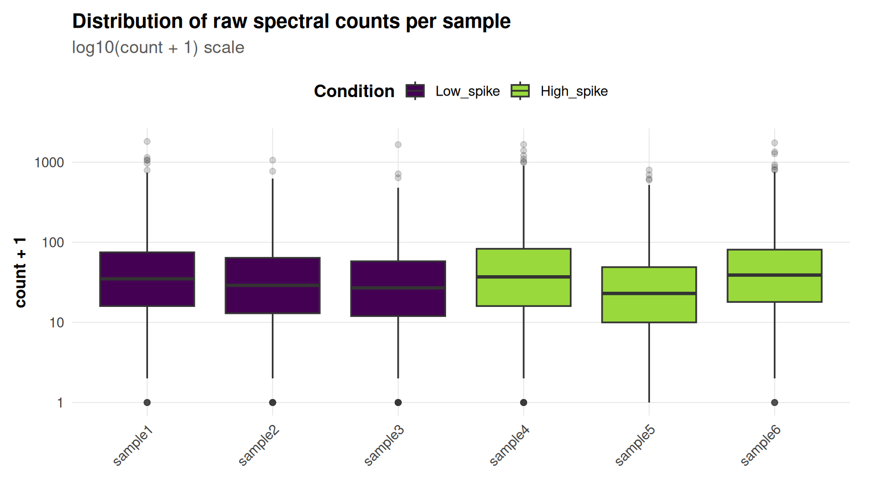
Before any modeling, it is good practice to look at the raw distribution of the counts, and at the total sequencing/spectral depth per sample.
```{r, fig.width=9, fig.height=5}
count_matrix %>%
  as.data.frame() %>%
  rownames_to_column("protein") %>%
  pivot_longer(-protein, names_to = "sample", values_to = "count") %>%
  left_join(rownames_to_column(col_data, "sample"), by = "sample") %>%
  ggplot(aes(x = sample, y = count + 1, fill = condition)) +
  geom_boxplot(outlier.alpha = 0.2) +
  scale_y_log10() +
  scale_fill_viridis_d(option = "D", end = 0.85) +
  labs(title = "Distribution of raw spectral counts per sample",
       subtitle = "log10(count + 1) scale",
       x = NULL, y = "count + 1", fill = "Condition") +
  theme_proteo() +
  theme(axis.text.x = element_text(angle = 45, hjust = 1))
```
::: {.callout-tip title="Interpretation"}
Differences in the overall level (median, spread) between samples of the same condition reflect technical variation in MS acquisition depth — exactly what the DESeq2 size factors are meant to correct for before any statistical comparison is made.
:::
### Building the DESeqDataSet and running the standard workflow
```{r}
dds <- DESeqDataSetFromMatrix(
  countData = count_matrix,
  colData   = col_data,
  design    = ~ condition
)

## Light pre-filtering: remove proteins with essentially no signal across
## all samples, before any normalization or dispersion estimation.
dds <- dds[rowSums(counts(dds)) >= 10, ]
```
The single wrapper `DESeq()` runs, in order: (1) estimation of the size factors $\hat{s}_j$ (`estimateSizeFactors`), (2) estimation and empirical Bayes shrinkage of the dispersions $\hat{\alpha}_i$ (`estimateDispersions`, fitting a **parametric** mean-dispersion trend by default — see the [theory section](#theory)), and (3) fitting of the NB-GLM and the Wald test on $\beta_i$ (`nbinomWaldTest`):
```{r}
dds <- DESeq(dds)
```
::: {.callout-note collapse="true" title="What if the parametric trend fails to fit? (a common occurrence on real data)"}
On real, especially noisier or coarser-count proteomics data, this exact call can raise: *"all gene-wise dispersion estimates are within 2 orders of magnitude from the minimum value, and so the standard curve fitting techniques will not work."* This happens when the per-protein dispersion estimates lack enough dynamic range for a parametric curve to be identifiable — DESeq2 deliberately refuses to fit one rather than silently returning an unreliable trend. It is not a bug to work around blindly, but a diagnostic signal about the input data. The standard, DESeq2-documented responses, in order of preference, are:
```r
## 1) Retry with a more flexible local-regression trend:
dds <- DESeq(dds, fitType = "local")

## 2) If that also fails, fall back to the gene-wise estimates as final
##    (no trend shrinkage at all):
dds <- estimateSizeFactors(dds)
dds <- estimateDispersionsGeneEst(dds)
dispersions(dds) <- mcols(dds)$dispGeneEst
dds <- nbinomWaldTest(dds)
```
This does not arise with the simulated data used in this tutorial (calibrated to have realistic dynamic range by construction), but it is worth recognizing on sight rather than mistaking it for a coding error.
:::
```{r}
sizeFactors(dds) %>%
  round(3) %>%
  as.data.frame() %>%
  setNames("Size factor") %>%
  kable(caption = "Table 1: Estimated size factors per sample")
```
### Exploratory analysis on the variance-stabilized data
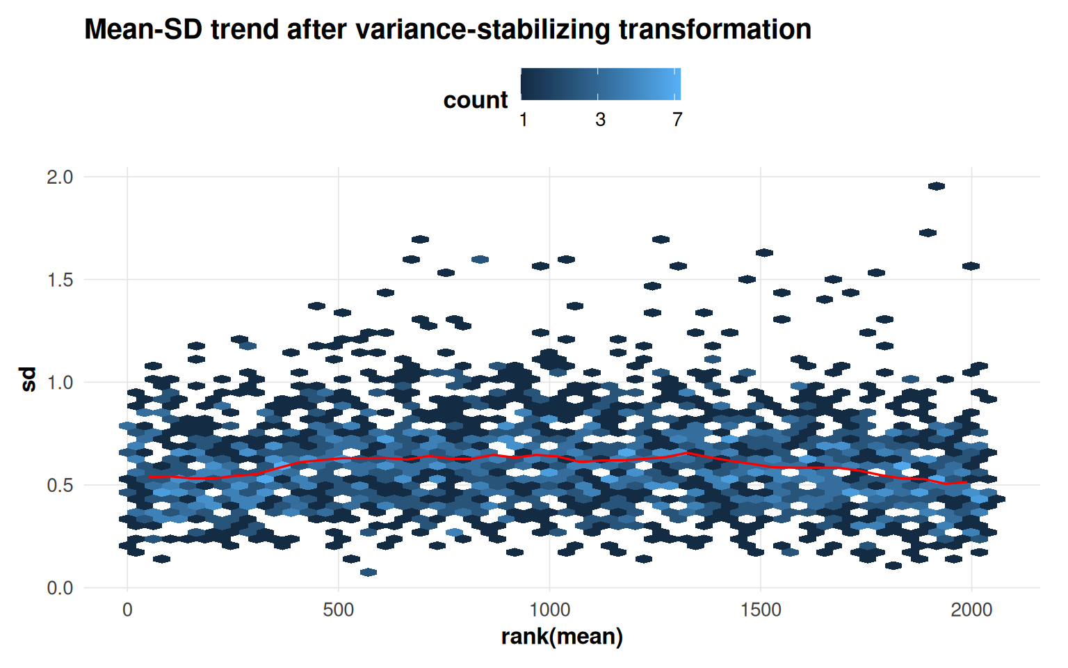
For visualization purposes only (never for the actual differential test, which always uses the raw counts), DESeq2 provides a **variance-stabilizing transformation (VST)**, which removes the mean-variance dependence characteristic of count data so that Euclidean-distance-based methods (PCA, hierarchical clustering) become meaningful.
```{r}
vsd <- vst(dds, blind = TRUE)
```
::: {.callout-note collapse="true" title="What if vst() refuses to run? (a common occurrence on real data)"}
`vst()` uses a fast heuristic: it fits its internal trend on a random subsample of proteins with mean normalized count above 5. On coarser or lower-count real data, too few proteins may clear that threshold, and `vst()` will explicitly error out rather than silently returning a poor transformation, recommending either `varianceStabilizingTransformation()` directly, or — the lightest fallback — `normTransform(dds)`, a simple log2(normalized count + 1) transform that needs no dispersion-trend fitting at all and is perfectly adequate for *exploratory* PCA/heatmap plots (never for the actual statistical test, which always uses the raw counts regardless). As with the dispersion-trend fitting above, this does not arise with the well-behaved simulated counts used here, but is useful to recognize on real data.
:::
::: panel-tabset
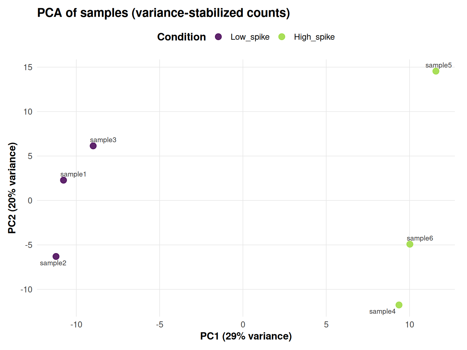
#### PCA
```{r, fig.width=8, fig.height=6}
plot_pca_proteo(vsd, intgroup = "condition",
                 title = "PCA of samples (variance-stabilized counts)")
```
#### Sample-to-sample distances
```{r, fig.width=8, fig.height=6}
sample_dists <- dist(t(SummarizedExperiment::assay(vsd)))

as.matrix(sample_dists) %>%
  as.data.frame() %>%
  rownames_to_column("sample1") %>%
  pivot_longer(-sample1, names_to = "sample2", values_to = "distance") %>%
  ggplot(aes(x = sample1, y = sample2, fill = distance)) +
  geom_tile() +
  scale_fill_viridis_c(option = "C", direction = -1) +
  labs(title = "Sample-to-sample Euclidean distances", x = NULL, y = NULL, fill = "Distance") +
  theme_proteo() +
  theme(axis.text.x = element_text(angle = 45, hjust = 1))
```
#### Mean-SD trend
```{r, fig.width=8, fig.height=5}
vsn::meanSdPlot(SummarizedExperiment::assay(vsd), plot = FALSE)$gg +
  labs(title = "Mean-SD trend after variance-stabilizing transformation") +
  theme_proteo()
```
:::
::: {.callout-tip title="Interpretation"}
On the PCA plot, samples are expected to separate along PC1 (or PC2) mainly by **condition** (spike-in level) if the experimental effect dominates technical noise; a flat mean-SD trend confirms that the VST has successfully removed the count-data mean-variance dependence, validating its use for the exploratory plots above.
:::
## Application: Differential Analysis Step by Step
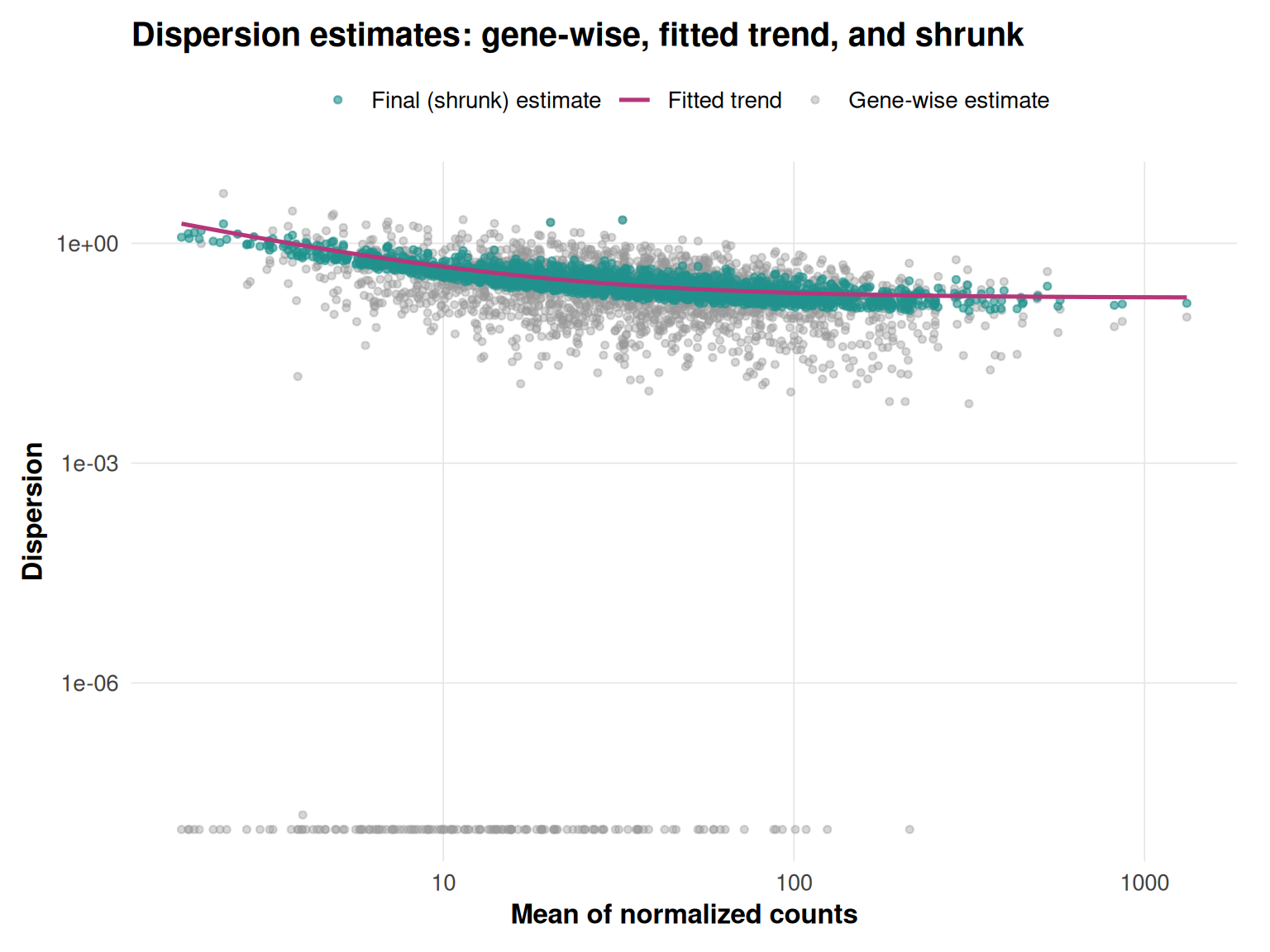
### Dispersion estimation diagnostic
```{r, fig.width=8, fig.height=6}
plot_dispersions(dds, title = "Dispersion estimates: gene-wise, fitted trend, and shrunk")
```
::: {.callout-tip title="Reading this plot"}
Gray points are the raw per-protein MLE dispersions; the pink line is the fitted mean-dispersion trend $\alpha_{\text{trend}}(\mu)$; teal points are each protein's **final, shrunk** dispersion actually used for testing. A trend that decreases with the mean count, and final estimates pulled toward it, indicate the empirical Bayes shrinkage is behaving as expected (see the [theory section](#theory)).
:::
### Extracting results and shrinking log2 fold changes
```{r}
res <- results(dds, contrast = c("condition", levels(col_data$condition)[2], levels(col_data$condition)[1]),
                alpha = 0.05)

## Shrink the log2 fold changes with the adaptive apeglm estimator, for
## more reliable ranking, MA plots and volcano plots (see theory section).
coef_name <- resultsNames(dds)[grepl("condition", resultsNames(dds))]
res_shrunk <- lfcShrink(dds, coef = coef_name, type = "apeglm")

summary(res)
```
```{r}
res_shrunk %>%
  deseq_table(caption = "Table 2: Top 15 differential proteins (shrunk log2 fold changes, ranked by adjusted p-value)")
```
### Visualizing the results
::: panel-tabset
#### Volcano plot
```{r, fig.width=9, fig.height=7}
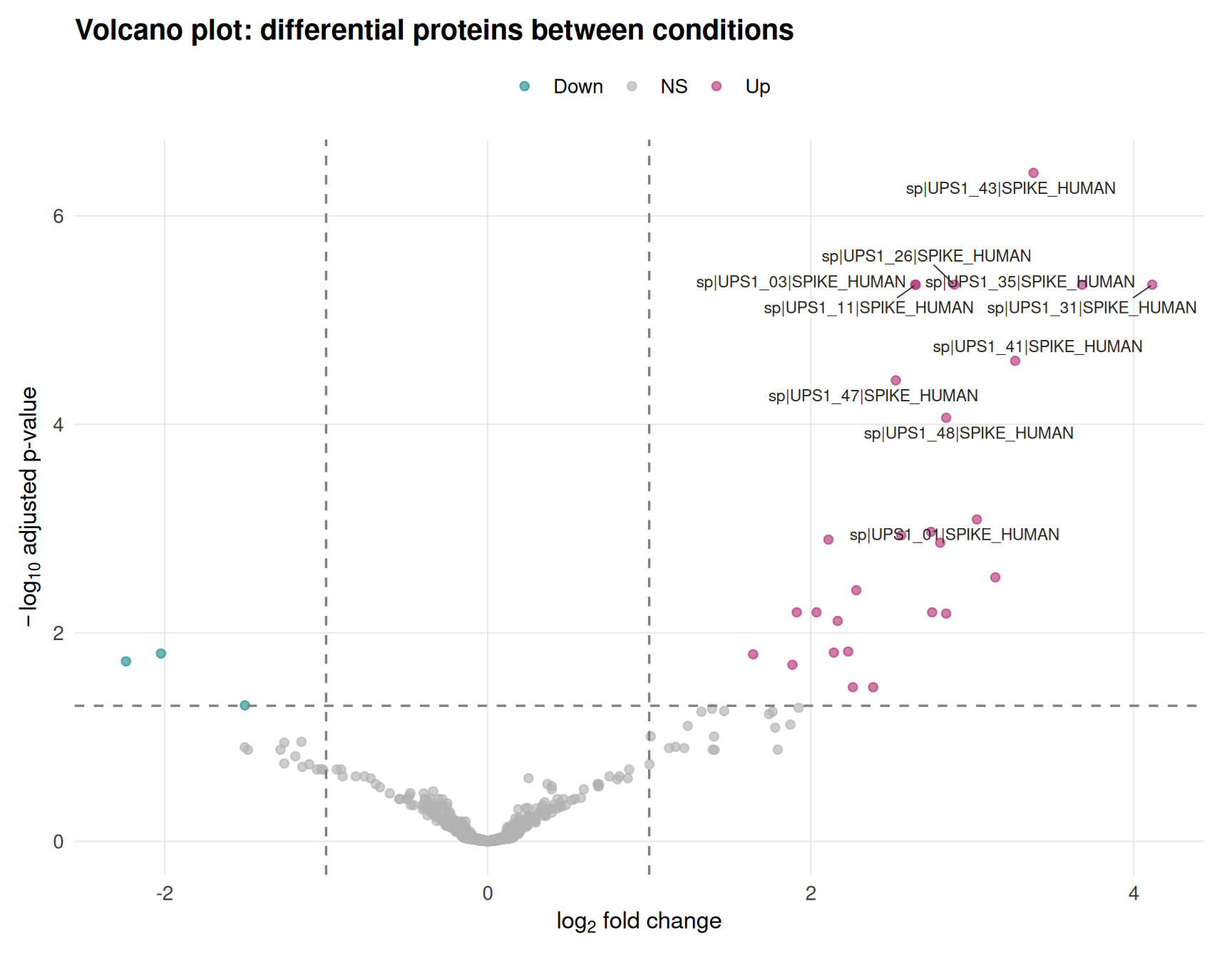
plot_volcano(as.data.frame(res_shrunk), lfc_thresh = 1, alpha = 0.05,
             title = "Volcano plot: differential proteins between conditions")
```
#### MA plot
```{r, fig.width=9, fig.height=6}
plot_ma(as.data.frame(res_shrunk), lfc_thresh = 1, alpha = 0.05,
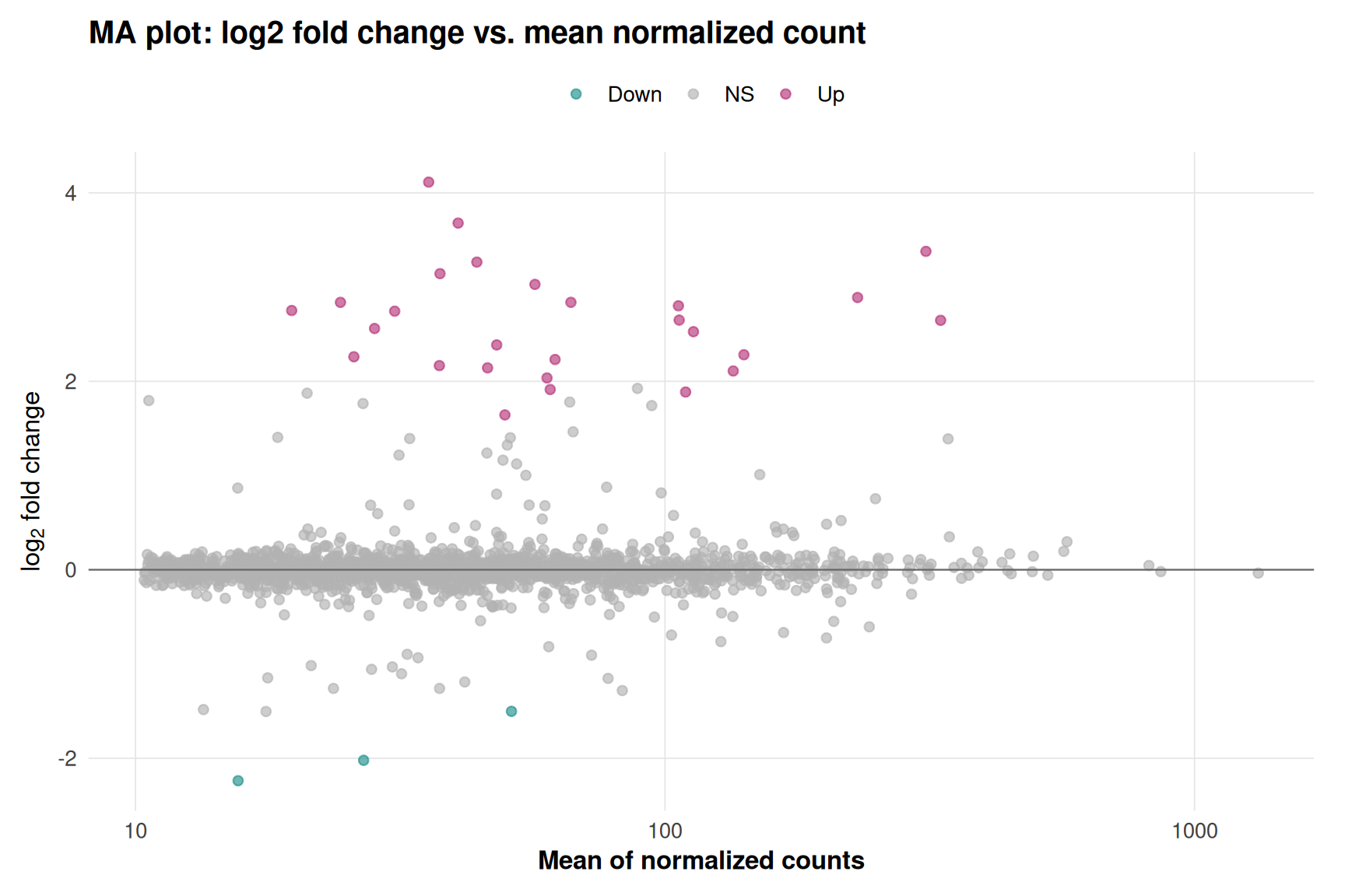
         title = "MA plot: log2 fold change vs. mean normalized count")
```
#### Heatmap of the top differential proteins
```{r, fig.width=9, fig.height=8}
top_proteins <- as.data.frame(res_shrunk) %>%
  rownames_to_column("protein") %>%
  filter(!is.na(padj)) %>%
  arrange(padj) %>%
  slice_head(n = 30) %>%
  pull(protein)

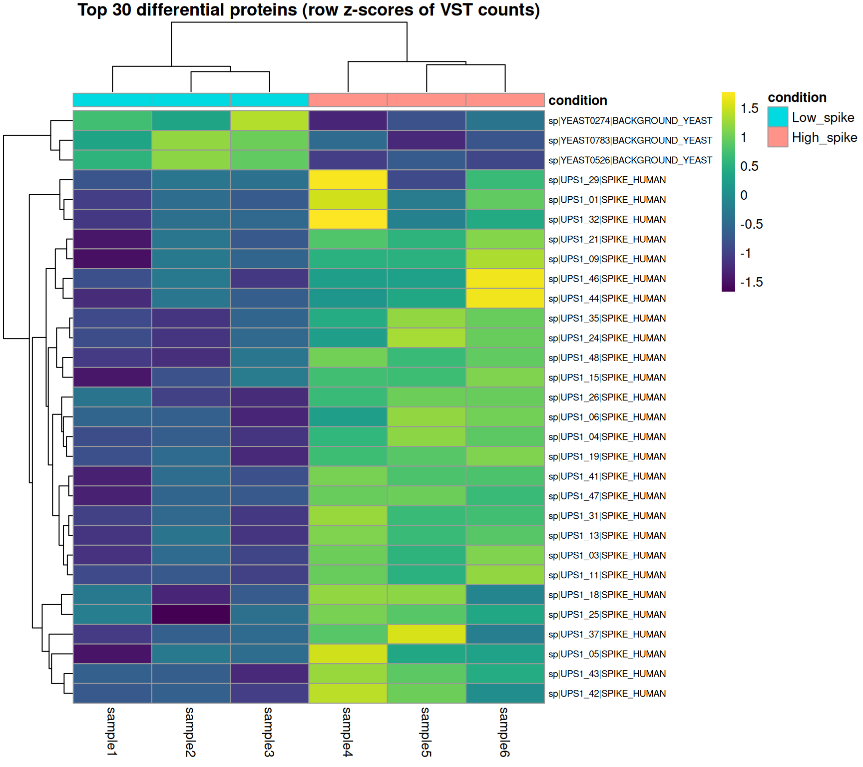
heat_data <- SummarizedExperiment::assay(vsd)[top_proteins, ]
heat_data <- t(scale(t(heat_data)))  ## z-score per protein across samples

pheatmap(
  heat_data,
  annotation_col = col_data,
  color = viridis(100),
  show_rownames = TRUE,
  fontsize_row = 7,
  main = "Top 30 differential proteins (row z-scores of VST counts)"
)
```
:::
::: {.callout-tip title="Interpretation"}
On the volcano and MA plots, points colored as "Up"/"Down" correspond to proteins with $|\log_2 \text{FC}| > 1$ and adjusted p-value $< 0.05$. On the heatmap, a clean block structure — differential proteins clustering strongly by condition — is the visual signature of a successful differential analysis; the annotation strip confirms this matches the known experimental condition rather than some unrelated batch effect.
:::
### Checking against the known ground truth
Because the UPS1 proteins are, by design, the only proteins expected to differ between conditions, this dataset allows an actual, quantitative check of the method's performance — something essentially never possible with a purely biological dataset.
```{r}
## The 48 Sigma UPS1 proteins are human recombinant standards spiked into
## a yeast background; UniProt-style FASTA headers used in this benchmark
## therefore tag UPS1 proteins with a "_HUMAN" suffix and yeast background
## proteins with a "_YEAST" suffix -- a simple, reliable ground-truth flag
## that requires no extra metadata file.
is_ups1 <- grepl("HUMAN", rownames(res_shrunk), ignore.case = TRUE)

truth_table <- as.data.frame(res_shrunk) %>%
  mutate(
    truth = ifelse(is_ups1, "UPS1 (true positive)", "Yeast background (true negative)"),
    called_de = !is.na(padj) & padj < 0.05
  ) %>%
  count(truth, called_de)
truth_table %>%
  kable(caption = "Table 3: Confusion table of DESeq2 calls against the known spike-in ground truth")
```
::: {.callout-important title="How to read this diagnostic"}
A high proportion of UPS1 proteins correctly called differential (**sensitivity**), together with a low proportion of yeast background proteins incorrectly called differential (**false-positive rate**), is direct empirical evidence that the DESeq2 negative-binomial workflow is well calibrated on this dataset. A markedly inflated false-positive rate among yeast proteins would instead be a warning sign that the count model is not well suited to this particular data (see the state-of-the-art caveats above), and would justify comparing against a proteomics-native method such as `DEqMS` or `MSstats` [@vega2020deqms; @langley2015comparative].
:::
## Model Diagnostics and Limits of This Analysis {#limits}
::: {.callout-note collapse="true" title="Limitations of this tutorial, and of count-based proteomics workflows in general"}
- **Simulated counts.** The dataset used above is simulated, calibrated to the real design and realistic spectral-count scales of Ramus et al. (2016) [@ramus2016spiked], but is not itself a real acquisition. This was a deliberate choice (see the [dataset section](#dataset)) so that the standard `DESeq2` functions could be demonstrated exactly as documented; a real acquisition can be substituted with no change beyond the import step, but may trigger the fitting issues flagged in the callouts above.
- **Small number of replicates.** With only 3 replicates per condition (as here, and as is typical of most proteomics experiments), dispersion estimates — even after empirical Bayes shrinkage — remain less stable than in a large RNA-seq cohort; this is precisely why the shrinkage machinery of the [theory section](#theory) matters so much here.
- **Independent-filtering threshold.** The low-count filtering step should always be inspected (via `plotMA()`-style diagnostics or the p-value histogram) rather than left at default settings, given the naturally lower counts of proteomics data <cite index="6-1">compared to RNA-seq</cite>.
- **No missing-value model.** DESeq2 has no explicit model for missing-not-at-random values; this is not an issue for genuine spectral counts (a true zero is a valid observation), but would be a serious limitation if this workflow were applied instead to LFQ-intensity-derived pseudo-counts, as discussed in the [state-of-the-art section](#dataset).
:::
## Results
Applied to the yeast/UPS1 spike-in benchmark of Ramus et al. (2016) [@ramus2016spiked], the DESeq2 negative-binomial workflow recovers the spiked-in human UPS1 proteins as the dominant class of differentially abundant proteins between spike-in levels, consistently with the experimental ground truth, while the constant yeast background is overwhelmingly retained as non-differential after Benjamini–Hochberg FDR control. This constitutes direct empirical support, on real data with known truth, for the broader literature finding that DESeq2 <cite index="6-1">performs comparatively well</cite> among count-based differential-expression methods applied to proteomics data — while the diagnostics and limitations discussed above make clear that this performance should always be checked, on each new dataset, rather than assumed by analogy with RNA-seq.
Methodologically, this tutorial illustrates the general count-based differential-proteomics workflow: (1) recover or construct a genuine integer count matrix (spectral/PSM counts, not intensities), (2) normalize with the median-of-ratios estimator, robust to the very kind of massive, designed differential effect present in a spike-in study, (3) estimate dispersions with empirical Bayes shrinkage to compensate for small replicate numbers, (4) test with the Wald statistic and shrink the fold changes with `apeglm`, and (5) always control the false discovery rate on `padj`, never on the raw p-value.
::: {.callout-tip title="Key takeaways"}
- DESeq2's negative-binomial model was built for RNA-seq, but it transfers to any genuine **integer count** matrix — including proteomics **spectral/PSM counts** — with no change to the underlying mathematics.
- It is **not** appropriate for continuous, already-normalized quantities such as LFQ intensities or iBAQ values, which violate the discreteness assumption at the core of the model.
- Because proteomics counts are typically smaller and noisier than RNA-seq counts, dispersion shrinkage, independent filtering and fold-change shrinkage (`apeglm`) matter proportionally more, not less.
- Whenever possible, validate the workflow on a dataset with a **known ground truth** (such as a spike-in benchmark) before trusting it on a purely exploratory biological comparison.
- Always report and interpret the **adjusted** p-value (`padj`, Benjamini–Hochberg FDR), never the raw p-value.
:::
## Computational informations
<details>
<summary>Session informations</summary>
```{r session_info, results='markup'}
devtools::session_info()
```
</details>