library("corrkit")
d <- simulate_cor_data(150)
cc <- cor_compute(d, x = c("CRP", "IL6", "BDNF", "NfL", "BIN_CRP"),
y = c("depression", "fatigue", "cognition"), labels = attr(d, "labels"))
plot_cor_forest(cc)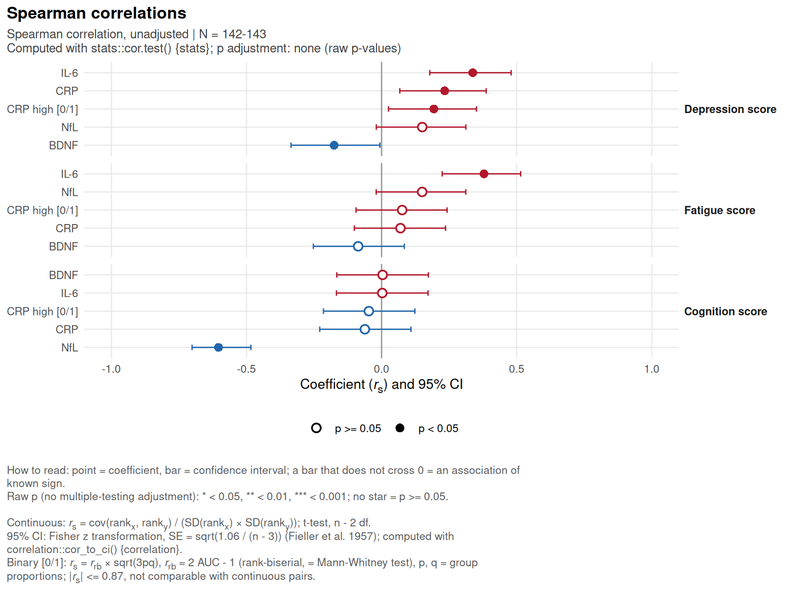
One row per pair: point = coefficient, bar = confidence interval, filled point = p (adjusted if requested) below alpha. A cross analysis has one panel per y (e.g. per score); a matrix analysis lists every pair. Complements the heatmap: the heatmap shows the structure, the forest plot shows the precision of each coefficient.
plot_cor_forest(
  x,
  labels = NULL,
  use_adj = TRUE,
  alpha = 0.05,
  sort = TRUE,
  base_size = 10,
  title = NULL,
  palette = COR_PAL,
  show_note = TRUE,
  caption_width = 110
)
x
|
output of cor_compute()
|
labels
|
named vector variable -> label (default: the labels given to cor_compute())
|
use_adj
|
filled points from adjusted (TRUE) or raw p-values
|
alpha
|
significance threshold of the filled points |
sort
|
sort the pairs by coefficient within each panel |
base_size
|
base font size |
title
|
title (default " |
palette
|
colours of the negative / positive coefficients (named low / high) |
show_note
|
add the binary-variable line to the caption |
caption_width
|
wrap the caption lines at this number of characters (NULL = no wrapping)
|
a ggplot
plot() on a cor_compute() result, which calls this function for type = “forest”.
library("corrkit")

d  <- simulate_cor_data(150)
cc <- cor_compute(d, x = c("CRP", "IL6", "BDNF", "NfL", "BIN_CRP"),
                  y = c("depression", "fatigue", "cognition"), labels = attr(d, "labels"))
plot_cor_forest(cc)