Exercice 9 – Statistique en grande dimension

On souhaite réaliser une petite étude par simulation pour évaluer les qualités respectives de 4 méthodes d’estimation d’un modèle de régression linéaire. On s’intéresse pour chacune d’elle à ses qualités de sélection de variables et à ses qualités prédictives. Le programme SimusReg.R permet de réaliser cette étude. Il contient deux fonctions, Simudata et la fonction principale fun, et un exemple d’utilisation en fin de programme.

Show the code

n = 100
p = 500
X = matrix(rnorm(n*p), n, p)

Show the code

library(lars)

Loaded lars 1.3


Attachement du package : 'lars'

L'objet suivant est masqué depuis 'package:psych':

    error.bars

Show the code

library(leaps)
library(glmnet)

Le chargement a nécessité le package : Matrix

Loaded glmnet 4.1-8

Show the code

DataSimulation = function(n,p){
  if(p < 4){stop("p>3 require")}
  # We create our matrix of explanatory variables
  X = matrix(rnorm(n*p), n, p)
  
  # We define our coefficients of regression 
  coeff = matrix(0, p)
  coeff[1:3] = 2
  
  # We build our explanatory variables
  y = X%*%coeff + rnorm(n, sd = 2)
  return(list(X = X, y = y, coeff = coeff))
}



fun = function(n, p, M = 100){ # By default, we make M = 100 simulation 
  
  ## Initialization 
  #################
  selec_method1 = NULL; selec_method2 = NULL; selec_method3 = NULL;
  taille_method1 = NULL; taille_method2 = NULL; taille_method3 = NULL;
  prev_method1 = NULL; prev_method2 = NULL; prev_method3 = NULL; prev_method4 = NULL;
  temps1 = NULL; temps2 = NULL; temps3 = NULL; temps4 = NULL;
  
  for(i in 1:M){
    cat(paste(i, ":")) # counter to see progress
    
    # We define our train set
    datatrain = DataSimulation(n, p)
    Xtrain = datatrain$X
    y = datatrain$y
    coeff = datatrain$coeff
    
    # We define our test set
    datatest = DataSimulation(n, p)
    Xtest = datatest$X
    ytest = datatest$y
    
    
    ## Regression 
    #################
    
    # Method 1 : Forward-Hybrid with BIC
    tic = proc.time()
    tab = data.frame(y = y, X = Xtrain)
    fit0 = lm(y~1, tab)
    fit = lm(y~., tab)
    tmp = step(fit0, scope = formula(fit),
               k = log(n), # BIC criteria
               direction = "both", # Hybrid
               trace = 0)
    noms = sort(names(tmp$model))
    selec_method1[i] = identical(
      noms[-length(noms)], sort(paste("X.", which(coeff != 0), sep = ""))
      )
    taille_method1[i] = length(noms) - 1
    prev_method1[i] = mean((predict(tmp,data.frame(X = Xtest)) - ytest)^2)
    tac = proc.time() - tic
    temps1[i] = tac[3]
    
    # Method 2 : Lasso
    tic = proc.time()
    cvglm = cv.glmnet(Xtrain, y) # By default we have Lasso
    lambda = cvglm$lambda.min
    coef2 = coef(cvglm, s = lambda)[-1]
    index = which(coef2 != 0) 
    selec_method2[i] = identical(sort(index), which(coeff != 0))
    taille_method2[i] = length(index)
    prev_method2[i] = mean((predict(cvglm, Xtest, s = lambda) - ytest)^2)
    tac = proc.time() - tic
    temps2[i] = tac[3]
    
    # Methods 3 and 4 : Adaptive Lasso and  Gauss-Lasso  
    if(length(index) == 0){
      selec_method3[i] = selec_method2[i]
      taille_method3[i] = taille_method2[i]
      prev_method3[i] = prev_method2[i]
      prev_method4[i] = prev_method2[i]}
    else{
      # Adaptive Lasso part
      cvglm = cv.glmnet(Xtrain, y,
                        penalty.factor = 1/abs(coef2))
      lambda = cvglm$lambda.min
      coef3 = coef(cvglm, s = lambda)[-1]
      index = which(coef3 != 0) 
      selec_method3[i] = identical(sort(index), which(coeff != 0))
      taille_method3[i] = length(index)
      prev_method3[i] = mean((predict(cvglm, Xtest, s = lambda) - ytest)^2)
      tac = proc.time() - tic
      temps3[i] = tac[3]
      
      # Gauss-Lasso part
      if(length(index) == 0){
        prev_method4[i] = mean((mean(y) - ytest)^2)}
      else{
        tab = data.frame(y = y, X = Xtrain)
        reg = lm(y~., 
                 data = tab[, c(1, index + 1)])
        prev_method4[i] = mean((predict(reg, data.frame(X = Xtest)) - ytest)^2)
        tac = proc.time() - tic
        temps4[i] = tac[3]
      }
    }
  }
  
  ## Results
  #################
  res = list(mean(selec_method1), mean(selec_method2), mean(selec_method3), taille_method1, taille_method2, taille_method3, prev_method1, prev_method2, prev_method3, prev_method4, mean(temps1), mean(temps2), mean(temps3), mean(temps4))
  
  names(res) = c("selec_method1", "selec_method2", "selec_method3", "taille_method1", "taille_method2", "taille_method3", "prev_method1", "prev_method2", "prev_method3", "prev_method4", "temps1", "temps2", "temps3", "temps4")
  
  return(res)
}

fun2 = function(n, p, M = 100){ # By default, we make M = 100 simulation 
  
  ## Initialization 
  #################
  selec_method1 = NULL; selec_method2 = NULL; selec_method3 = NULL;
  taille_method1 = NULL; taille_method2 = NULL; taille_method3 = NULL;
  prev_method1 = NULL; prev_method2 = NULL; prev_method3 = NULL; prev_method4 = NULL;
  temps1 = NULL; temps2 = NULL; temps3 = NULL; temps4 = NULL;
  
  for(i in 1:M){
    cat(paste(i, ":")) # counter to see progress
    
    # We define our train set
    datatrain = DataSimulation(n, p)
    Xtrain = datatrain$X
    y = datatrain$y
    coeff = datatrain$coeff
    
    # We define our test set
    datatest = DataSimulation(n, p)
    Xtest = datatest$X
    ytest = datatest$y
    
    
    ## Regression 
    #################
    
    # Method 2 : Lasso
    tic = proc.time()
    cvglm = cv.glmnet(Xtrain, y) # By default we have Lasso
    lambda = cvglm$lambda.min
    coef2 = coef(cvglm, s = lambda)[-1]
    index = which(coef2 != 0) 
    selec_method2[i] = identical(sort(index), which(coeff != 0))
    taille_method2[i] = length(index)
    prev_method2[i] = mean((predict(cvglm, Xtest, s = lambda) - ytest)^2)
    tac = proc.time() - tic
    temps2[i] = tac[3]
    
    # Methods 3 and 4 : Adaptive Lasso and  Gauss-Lasso  
    if(length(index) == 0){
      selec_method3[i] = selec_method2[i]
      taille_method3[i] = taille_method2[i]
      prev_method3[i] = prev_method2[i]
      prev_method4[i] = prev_method2[i]}
    else{
      # Adaptive Lasso part
      cvglm = cv.glmnet(Xtrain, y,
                        penalty.factor = 1/abs(coef2))
      lambda = cvglm$lambda.min
      coef3 = coef(cvglm, s = lambda)[-1]
      index = which(coef3 != 0) 
      selec_method3[i] = identical(sort(index), which(coeff != 0))
      taille_method3[i] = length(index)
      prev_method3[i] = mean((predict(cvglm, Xtest, s = lambda) - ytest)^2)
      tac = proc.time() - tic
      temps3[i] = tac[3]
      
      # Gauss-Lasso part
      if(length(index) == 0){
        prev_method4[i] = mean((mean(y) - ytest)^2)}
      else{
        tab = data.frame(y = y, X = Xtrain)
        reg = lm(y~., 
                 data = tab[, c(1, index + 1)])
        prev_method4[i] = mean((predict(reg, data.frame(X = Xtest)) - ytest)^2)
        tac = proc.time() - tic
        temps4[i] = tac[3]
      }
    }
  }
  
  ## Results
  #################
  res = list(mean(selec_method1), mean(selec_method2), mean(selec_method3), taille_method1, taille_method2, taille_method3, prev_method1, prev_method2, prev_method3, prev_method4, mean(temps1), mean(temps2), mean(temps3), mean(temps4))
  
  names(res) = c("selec_method1", "selec_method2", "selec_method3", "taille_method1", "taille_method2", "taille_method3", "prev_method1", "prev_method2", "prev_method3", "prev_method4", "temps1", "temps2", "temps3", "temps4")
  
  return(res)
}

Show the code

###### Exemple
a=fun(50,5,100)

1 :2 :3 :4 :5 :6 :7 :8 :9 :10 :11 :12 :13 :14 :15 :16 :17 :18 :19 :20 :21 :22 :23 :24 :25 :26 :27 :28 :29 :30 :31 :32 :33 :34 :35 :36 :37 :38 :39 :40 :41 :42 :43 :44 :45 :46 :47 :48 :49 :50 :51 :52 :53 :54 :55 :56 :57 :58 :59 :60 :61 :62 :63 :64 :65 :66 :67 :68 :69 :70 :71 :72 :73 :74 :75 :76 :77 :78 :79 :80 :81 :82 :83 :84 :85 :86 :87 :88 :89 :90 :91 :92 :93 :94 :95 :96 :97 :98 :99 :100 :

Show the code

a$selec_method1

[1] 0.9

Show the code

a$selec_method2

[1] 0.16

Show the code

a$selec_method3

[1] 0.7

Show the code

a$taille_method1

  [1] 3 3 4 3 3 3 3 3 3 3 3 3 4 3 3 3 3 3 3 3 3 3 3 3 3 3 3 3 3 3 3 4 3 3 3 3 3
 [38] 3 3 4 3 3 3 3 4 3 3 3 3 3 3 3 3 3 3 3 3 3 3 3 3 3 3 3 4 3 3 3 4 3 3 3 3 3
 [75] 3 3 3 3 3 3 3 4 3 3 3 3 3 3 3 3 4 3 3 3 3 3 3 4 3 3

Show the code

a$taille_method2

  [1] 5 5 5 4 4 5 3 5 3 5 5 5 5 4 4 4 3 4 4 4 5 4 3 4 5 5 4 4 3 5 5 4 4 4 5 4 4
 [38] 5 4 5 5 5 5 4 5 5 4 4 5 3 5 4 5 5 5 3 3 4 5 4 4 5 4 3 5 4 5 3 5 4 4 4 5 5
 [75] 5 3 4 5 3 4 5 5 5 5 5 5 5 5 3 3 5 5 3 4 5 5 4 4 3 5

Show the code

a$taille_method3

  [1] 3 3 5 3 3 5 3 3 3 3 3 3 5 3 3 3 3 3 4 3 3 3 3 3 5 3 3 3 3 4 5 4 3 3 4 3 3
 [38] 4 3 4 3 3 3 3 5 5 3 3 3 3 3 4 3 4 3 3 3 3 5 3 4 4 3 3 4 3 3 3 4 4 3 3 3 4
 [75] 4 3 3 4 3 3 3 5 3 4 3 3 4 3 3 3 5 4 3 3 3 3 3 4 3 3

Show the code

boxplot(sqrt(a$prev_method1),sqrt(a$prev_method2),sqrt(a$prev_method3),sqrt(a$prev_method4),names=c("Method1","Method2","Method3","Method4"),main="Title")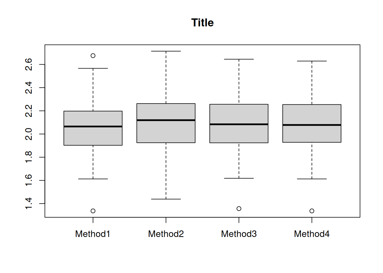

Show the code

mean(a$prev_method1)

[1] 4.317454

Show the code

mean(a$prev_method2)

[1] 4.482734

Show the code

mean(a$prev_method3)

[1] 4.405399

Show the code

mean(a$prev_method4)

[1] 4.397463

Show the code

a$temps1

[1] 0.01149

Show the code

a$temps2

[1] 0.02251

Show the code

a$temps3

[1] 0.04536

Show the code

a$temps4

[1] 0.04648

Question 1

Quel modèle génère la fonction Simudata ? Combien de variables explicatives sont générées ? Parmi elles, lesquelles sont pertinentes pour la modélisation ? Ecrire l’équation du modèle.

Question 2

Identifier les 4 méthodes d’estimation mises en oeuvre dans la fonction fun.

Question 3

Détailler les différentes sorties proposées par la fonction fun.

Question 4

Remplacer la valeur des options names et title du boxplot réalisé dans l’exemple par les bonnes informations.

Show the code

boxplot(sqrt(a$prev_method1),sqrt(a$prev_method2),sqrt(a$prev_method3),sqrt(a$prev_method4),
        names=c("Forward","Lasso","Adaptative Lasso","Gauss-Lasso"),
        main=paste("Erreur de prévision pour n =", 100,"et p=", 10),
        col = c("orchid3", "palegreen", "salmon2", "lightskyblue2"),
        ylim = c(1,3))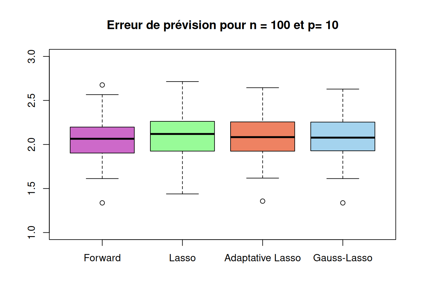

Question 5

Réaliser une étude comparative des méthodes lorsque \(n = 50\) et \(p = n/10\), \(p = n\), \(p = 2n\), \(p = 10n\). Pour chaque situation, on considèrera \(100\) simulations afin de calculer les différents critères. On synthétisera les résultats en terme de qualité de sélection, nombre de variables sélectionnées, erreurs de prévision et temps de calcul.

Show the code

#parallelisation
future::plan(multisession, workers = 2)

n = 50
p_list = c(n/10, n, 2*n, 10*n)

r_cas1 = fun(n, p_list[1])

1 :2 :3 :4 :5 :6 :7 :8 :9 :10 :11 :12 :13 :14 :15 :16 :17 :18 :19 :20 :21 :22 :23 :24 :25 :26 :27 :28 :29 :30 :31 :32 :33 :34 :35 :36 :37 :38 :39 :40 :41 :42 :43 :44 :45 :46 :47 :48 :49 :50 :51 :52 :53 :54 :55 :56 :57 :58 :59 :60 :61 :62 :63 :64 :65 :66 :67 :68 :69 :70 :71 :72 :73 :74 :75 :76 :77 :78 :79 :80 :81 :82 :83 :84 :85 :86 :87 :88 :89 :90 :91 :92 :93 :94 :95 :96 :97 :98 :99 :100 :

Show the code

r_cas2 = fun(n, p_list[2])

1 :2 :3 :4 :5 :6 :7 :8 :9 :10 :11 :12 :13 :14 :15 :16 :17 :18 :19 :20 :21 :22 :23 :24 :25 :26 :27 :28 :29 :30 :31 :32 :33 :34 :35 :36 :37 :38 :39 :40 :41 :42 :43 :44 :45 :46 :47 :48 :49 :50 :51 :52 :53 :54 :55 :56 :57 :58 :59 :60 :61 :62 :63 :64 :65 :66 :67 :68 :69 :70 :71 :72 :73 :74 :75 :76 :77 :78 :79 :80 :81 :82 :83 :84 :85 :86 :87 :88 :89 :90 :91 :92 :93 :94 :95 :96 :97 :98 :99 :100 :

Show the code

r_cas3 = fun(n, p_list[3])

1 :2 :

3 :

4 :

5 :

6 :

7 :

8 :

9 :

10 :

11 :

12 :

13 :14 :15 :

16 :17 :

18 :

19 :

20 :21 :

22 :23 :

24 :25 :

26 :

27 :28 :

29 :

30 :

31 :

32 :

33 :

34 :

35 :

36 :

37 :

38 :

39 :

40 :

41 :

42 :

43 :

44 :

45 :

46 :47 :

48 :

49 :50 :

51 :

52 :

53 :54 :

55 :

56 :57 :

58 :

59 :

60 :

61 :

62 :63 :

64 :

65 :

66 :

67 :

68 :69 :

70 :

71 :

72 :

73 :74 :

75 :76 :

77 :78 :79 :80 :

81 :

82 :

83 :

84 :

85 :

86 :

87 :

88 :

89 :

90 :

91 :

92 :93 :

94 :

95 :

96 :97 :

98 :99 :

100 :

Show the code

r_cas4 = fun(n, p_list[4],1)

1 :

Show the code

r_cas4bis = fun2(n, p_list[4])

1 :2 :3 :4 :5 :6 :7 :8 :9 :10 :11 :12 :13 :14 :15 :16 :17 :18 :19 :20 :21 :22 :23 :24 :25 :26 :27 :28 :29 :30 :31 :32 :33 :34 :35 :36 :37 :38 :39 :40 :41 :42 :43 :44 :45 :46 :47 :48 :49 :50 :51 :52 :53 :54 :55 :56 :57 :58 :59 :60 :61 :62 :63 :64 :65 :66 :67 :68 :69 :70 :71 :72 :73 :74 :75 :76 :77 :78 :79 :80 :81 :82 :83 :84 :85 :86 :87 :88 :89 :90 :91 :92 :93 :94 :95 :96 :97 :98 :99 :100 :

Show the code

# file_path <- file.path("../Data/r_cas1.rds")
# saveRDS(r_cas1, file = file_path)

# quit parallelisation
future::plan("sequential")

Show the code

# file_path <- file.path("../Data/r_cas1.rds")
# r_cas1 <- readRDS(file_path)

Show the code

res_cas1 = data.frame(
  Method = c("Forward", "Lasso", "Adaptative Lasso", "Gauss-Lasso"), 
  Quality_of_selection = c(r_cas1$selec_method1,r_cas1$selec_method2,r_cas1$selec_method3,NA),
  Mean_nb_selected_var = c(mean(r_cas1$taille_method1),mean(r_cas1$taille_method2),mean(r_cas1$taille_method3),NA),
  Prevision_error = c(mean(r_cas1$prev_method1),mean(r_cas1$prev_method2),mean(r_cas1$prev_method3),mean(r_cas1$prev_method4)),
  Running_time = c(r_cas1$temps1,r_cas1$temps2,r_cas1$temps3,r_cas1$temps4)
)
t(res_cas1)

                     [,1]       [,2]       [,3]               [,4]         
Method               "Forward"  "Lasso"    "Adaptative Lasso" "Gauss-Lasso"
Quality_of_selection "0.95"     "0.24"     "0.76"             NA           
Mean_nb_selected_var "3.05"     "4.19"     "3.29"             NA           
Prevision_error      "4.267999" "4.372448" "4.311278"         "4.298561"   
Running_time         "0.01006"  "0.02122"  "0.04285"          "0.04382"

Show the code

boxplot(sqrt(r_cas1$prev_method1),sqrt(r_cas1$prev_method2),sqrt(r_cas1$prev_method3),sqrt(r_cas1$prev_method4),
        names=c("Forward","Lasso","Adaptative Lasso","Gauss-Lasso"),
        main=paste("Erreur de prévision pour n =", n,"et p=", p_list[1]),
        col = c("orchid3", "palegreen", "salmon2", "lightskyblue2"))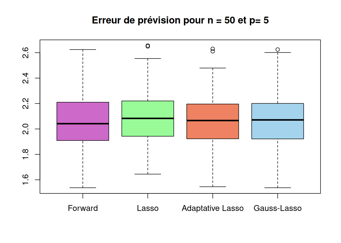

Show the code

res_cas2 = data.frame(
  Method = c("Forward", "Lasso", "Adaptative Lasso", "Gauss-Lasso"), 
  Quality_of_selection = c(r_cas2$selec_method1,r_cas2$selec_method2,r_cas2$selec_method3,NA),
  Mean_nb_selected_var = c(mean(r_cas2$taille_method1),mean(r_cas2$taille_method2),mean(r_cas2$taille_method3),NA),
  Prevision_error = c(mean(r_cas2$prev_method1),mean(r_cas2$prev_method2),mean(r_cas2$prev_method3),mean(r_cas2$prev_method4)),
  Running_time = c(r_cas2$temps1,r_cas2$temps2,r_cas2$temps3,r_cas2$temps4)
)
t(res_cas2)

                     [,1]       [,2]       [,3]               [,4]         
Method               "Forward"  "Lasso"    "Adaptative Lasso" "Gauss-Lasso"
Quality_of_selection "0.06"     "0.01"     "0.09"             NA           
Mean_nb_selected_var " 7.92"    "12.88"    " 8.17"            NA           
Prevision_error      "7.050225" "5.609938" "5.487207"         "6.401796"   
Running_time         "0.07149"  "0.04010"  "0.06590"          "0.06738"

Show the code

boxplot(sqrt(r_cas2$prev_method1),sqrt(r_cas2$prev_method2),sqrt(r_cas2$prev_method3),sqrt(r_cas2$prev_method4),
        names=c("Forward","Lasso","Adaptative Lasso","Gauss-Lasso"),
        main=paste("Erreur de prévision pour n =", n,"et p=", p_list[2]),
        col = c("orchid3", "palegreen", "salmon2", "lightskyblue2"))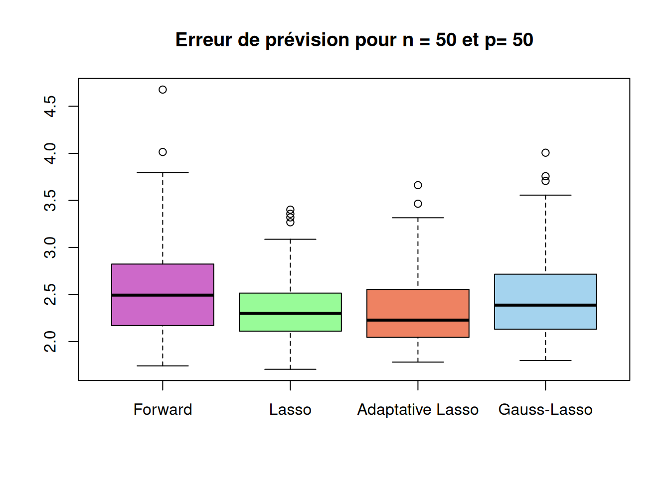

Show the code

res_cas3 = data.frame(
  Method = c("Forward", "Lasso", "Adaptative Lasso", "Gauss-Lasso"), 
  Quality_of_selection = c(r_cas3$selec_method1,r_cas3$selec_method2,r_cas3$selec_method3,NA),
  Mean_nb_selected_var = c(mean(r_cas3$taille_method1),mean(r_cas3$taille_method2),mean(r_cas3$taille_method3),NA),
  Prevision_error = c(mean(r_cas3$prev_method1),mean(r_cas3$prev_method2),mean(r_cas3$prev_method3),mean(r_cas3$prev_method4)),
  Running_time = c(r_cas3$temps1,r_cas3$temps2,r_cas3$temps3,r_cas3$temps4)
)
t(res_cas3)

                     [,1]        [,2]        [,3]               [,4]         
Method               "Forward"   "Lasso"     "Adaptative Lasso" "Gauss-Lasso"
Quality_of_selection "0.00"      "0.00"      "0.06"             NA           
Mean_nb_selected_var "40.57"     "15.80"     " 9.09"            NA           
Prevision_error      "16.207790" " 6.138163" " 5.738140"        " 6.723044"  
Running_time         "0.71804"   "0.04013"   "0.06882"          "0.07045"

Show the code

boxplot(sqrt(r_cas3$prev_method1),sqrt(r_cas3$prev_method2),sqrt(r_cas3$prev_method3),sqrt(r_cas3$prev_method4),
        names=c("Forward","Lasso","Adaptative Lasso","Gauss-Lasso"),
        main=paste("Erreur de prévision pour n =", n,"et p=", p_list[3]),
        col = c("orchid3", "palegreen", "salmon2", "lightskyblue2"))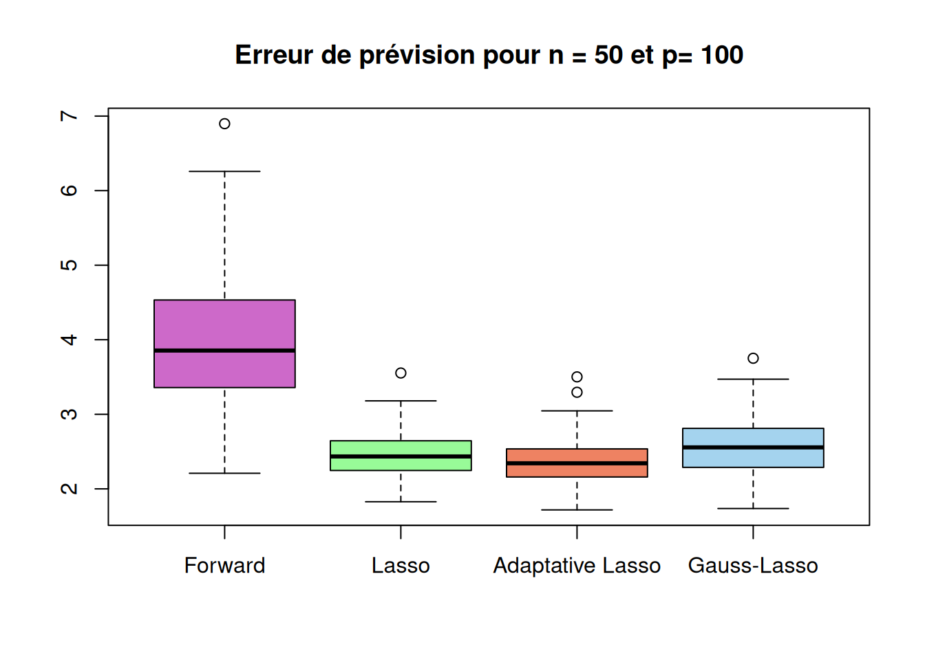

Show the code

res_cas4 = data.frame(
  Method = c("Forward", "Lasso", "Adaptative Lasso", "Gauss-Lasso"), 
  Quality_of_selection = c(r_cas4$selec_method1,r_cas4$selec_method2,r_cas4$selec_method3,NA),
  Mean_nb_selected_var = c(mean(r_cas4$taille_method1),mean(r_cas4$taille_method2),mean(r_cas4$taille_method3),NA),
  Prevision_error = c(mean(r_cas4$prev_method1),mean(r_cas4$prev_method2),mean(r_cas4$prev_method3),mean(r_cas4$prev_method4)),
  Running_time = c(r_cas4$temps1,r_cas4$temps2,r_cas4$temps3,r_cas4$temps4)
)
t(res_cas4)

                     [,1]        [,2]        [,3]               [,4]         
Method               "Forward"   "Lasso"     "Adaptative Lasso" "Gauss-Lasso"
Quality_of_selection " 0"        " 0"        " 0"               NA           
Mean_nb_selected_var "49"        "41"        "19"               NA           
Prevision_error      "11.762266" " 4.734249" " 4.562205"        " 5.403622"  
Running_time         "6.500"     "0.041"     "0.077"            "0.080"

Show the code

boxplot(sqrt(r_cas4$prev_method1),sqrt(r_cas4$prev_method2),sqrt(r_cas4$prev_method3),sqrt(r_cas4$prev_method4),
        names=c("Forward","Lasso","Adaptative Lasso","Gauss-Lasso"),
        main=paste("Erreur de prévision pour n =", n,"et p=", p_list[3]),
        col = c("orchid3", "palegreen", "salmon2", "lightskyblue2"))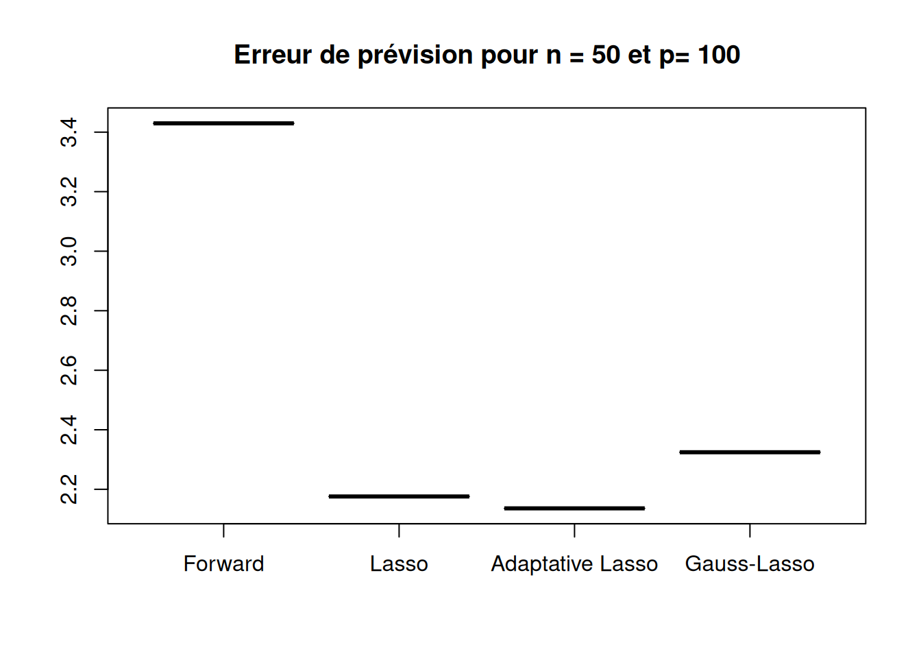

Show the code

res_cas4bis = data.frame(
  Method = c("Forward", "Lasso", "Adaptative Lasso", "Gauss-Lasso"), 
  Quality_of_selection = c(r_cas4bis$selec_method1,r_cas4bis$selec_method2,r_cas4bis$selec_method3,NA),
  Mean_nb_selected_var = c(mean(r_cas4bis$taille_method1),mean(r_cas4bis$taille_method2),mean(r_cas4bis$taille_method3),NA),
  Prevision_error = c(mean(r_cas4bis$prev_method1),mean(r_cas4bis$prev_method2),mean(r_cas4bis$prev_method3),mean(r_cas4bis$prev_method4)),
  Running_time = c(r_cas4bis$temps1,r_cas4bis$temps2,r_cas4bis$temps3,r_cas4bis$temps4)
)

Warning in mean.default(r_cas4bis$taille_method1): l'argument n'est ni
numérique, ni logique : renvoi de NA

Warning in mean.default(r_cas4bis$prev_method1): l'argument n'est ni numérique,
ni logique : renvoi de NA

Show the code

t(res_cas4bis)

                     [,1]      [,2]       [,3]               [,4]         
Method               "Forward" "Lasso"    "Adaptative Lasso" "Gauss-Lasso"
Quality_of_selection NA        "0.00"     "0.04"             NA           
Mean_nb_selected_var NA        "24.87"    "12.34"            NA           
Prevision_error      NA        "7.230664" "6.781834"         "7.861071"   
Running_time         NA        "0.04820"  "0.08404"          "0.08697"

Show the code

boxplot(sqrt(r_cas4$prev_method1),sqrt(r_cas4bis$prev_method2),sqrt(r_cas4bis$prev_method3),sqrt(r_cas4bis$prev_method4),
        names=c("Forward","Lasso","Adaptative Lasso","Gauss-Lasso"),
        main=paste("Erreur de prévision pour n =", n,"et p=", p_list[4]),
        col = c("orchid3", "palegreen", "salmon2", "lightskyblue2"))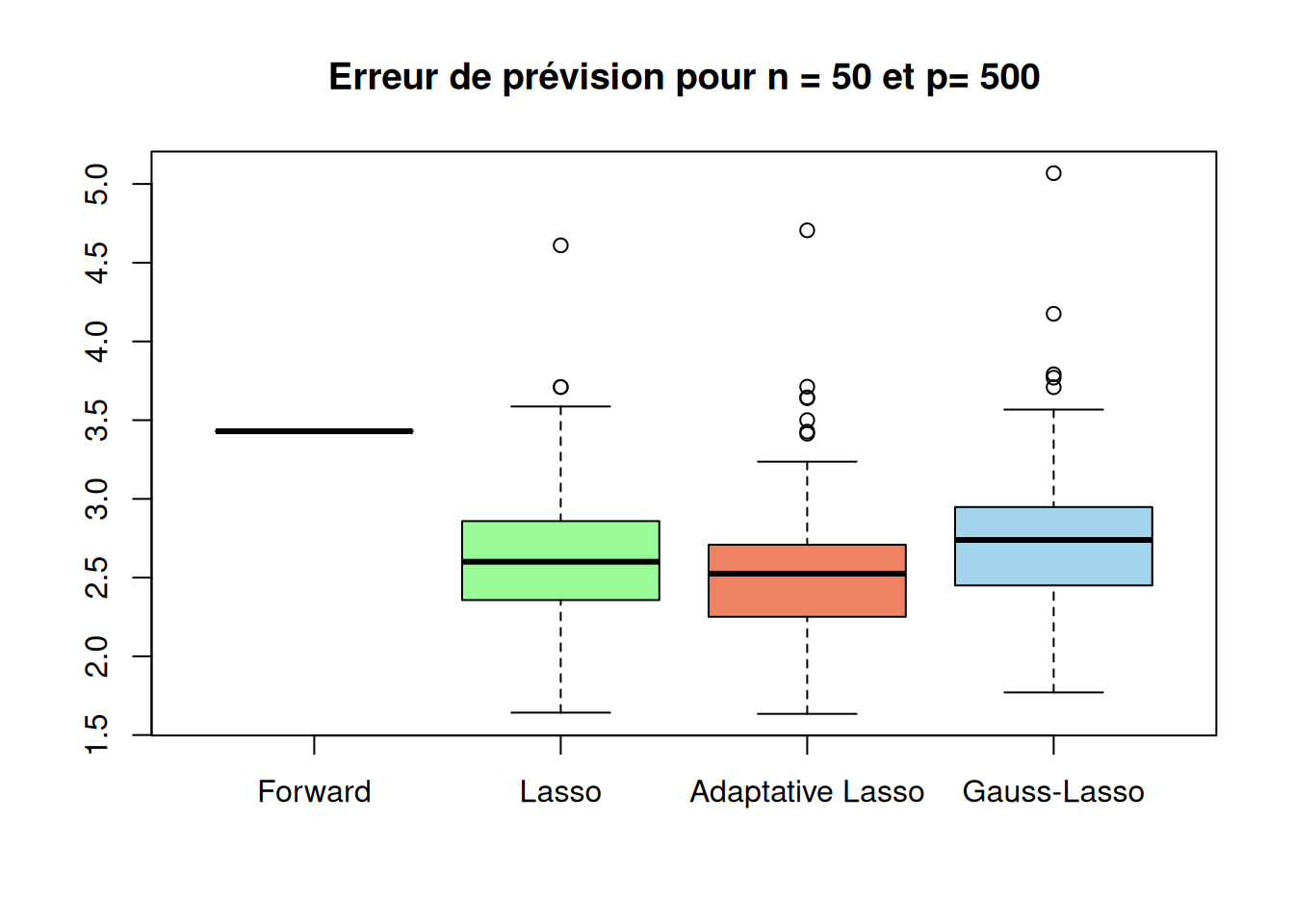

Question 6

Réaliser la même étude pour \(n = 100\) et \(p = n/10\), \(p = n\), \(p = 2n\), toujours basée sur \(100\) simulations dans chaque cas. Considérer de plus le cas \(p = 10n\) en ne faisant qu’une seule simulation afin d’en évaluer le temps de calcul. Une fois ce temps analysé, lancer \(100\) simulations pour \(p = 10n\) mais en omettant la méthode la plus couteuse en temps de calcul.

Show the code

#parallelisation
future::plan(multisession, workers = 2)

n = 100
p_list = c(n/10, n, 2*n, 10*n)

r_cas1 = fun(n, p_list[1])

1 :2 :3 :4 :5 :6 :7 :8 :9 :10 :11 :12 :13 :14 :15 :16 :17 :18 :19 :20 :21 :22 :23 :24 :25 :26 :27 :28 :29 :30 :31 :32 :33 :34 :35 :36 :37 :38 :39 :40 :41 :42 :43 :44 :45 :46 :47 :48 :49 :50 :51 :52 :53 :54 :55 :56 :57 :58 :59 :60 :61 :62 :63 :64 :65 :66 :67 :68 :69 :70 :71 :72 :73 :74 :75 :76 :77 :78 :79 :80 :81 :82 :83 :84 :85 :86 :87 :88 :89 :90 :91 :92 :93 :94 :95 :96 :97 :98 :99 :100 :

Show the code

r_cas2 = fun(n, p_list[2])

1 :2 :3 :4 :5 :6 :7 :8 :9 :10 :11 :12 :13 :14 :15 :16 :17 :18 :19 :20 :21 :22 :23 :24 :25 :26 :27 :28 :29 :30 :31 :32 :33 :34 :35 :36 :37 :38 :39 :40 :41 :42 :43 :44 :45 :46 :47 :48 :49 :50 :51 :52 :53 :54 :55 :56 :57 :58 :59 :60 :61 :62 :63 :64 :65 :66 :67 :68 :69 :70 :71 :72 :73 :74 :75 :76 :77 :78 :79 :80 :81 :82 :83 :84 :85 :86 :87 :88 :89 :90 :91 :92 :93 :94 :95 :96 :97 :98 :99 :100 :

Show the code

r_cas3 = fun(n, p_list[3])

1 :

2 :3 :4 :5 :6 :

7 :8 :9 :

10 :11 :

12 :

13 :14 :15 :16 :17 :18 :

19 :20 :

21 :

22 :23 :24 :25 :

26 :27 :

28 :29 :30 :

31 :

32 :33 :34 :

35 :

36 :37 :38 :39 :

40 :41 :42 :43 :

44 :

45 :46 :47 :

48 :

49 :

50 :51 :52 :

53 :54 :55 :56 :

57 :58 :

59 :

60 :61 :

62 :63 :

64 :

65 :66 :

67 :68 :

69 :

70 :71 :72 :73 :74 :

75 :

76 :77 :78 :

79 :80 :81 :82 :83 :

84 :85 :86 :87 :88 :89 :90 :

91 :

92 :93 :

94 :

95 :96 :97 :98 :

99 :100 :

Show the code

r_cas4 = fun(n, p_list[4],1)

1 :

Show the code

r_cas4bis = fun2(n, p_list[4])

1 :2 :3 :4 :5 :6 :7 :8 :9 :10 :11 :12 :13 :14 :15 :16 :17 :18 :19 :20 :21 :22 :23 :24 :25 :26 :27 :28 :29 :30 :31 :32 :33 :34 :35 :36 :37 :38 :39 :40 :41 :42 :43 :44 :45 :46 :47 :48 :49 :50 :51 :52 :53 :54 :55 :56 :57 :58 :59 :60 :61 :62 :63 :64 :65 :66 :67 :68 :69 :70 :71 :72 :73 :74 :75 :76 :77 :78 :79 :80 :81 :82 :83 :84 :85 :86 :87 :88 :89 :90 :91 :92 :93 :94 :95 :96 :97 :98 :99 :100 :

Show the code

# quit parallelisation
future::plan("sequential")

Show the code

res_cas1 = data.frame(
  Method = c("Forward", "Lasso", "Adaptative Lasso", "Gauss-Lasso"), 
  Quality_of_selection = c(r_cas1$selec_method1,r_cas1$selec_method2,r_cas1$selec_method3,NA),
  Mean_nb_selected_var = c(mean(r_cas1$taille_method1),mean(r_cas1$taille_method2),mean(r_cas1$taille_method3),NA),
  Prevision_error = c(mean(r_cas1$prev_method1),mean(r_cas1$prev_method2),mean(r_cas1$prev_method3),mean(r_cas1$prev_method4)),
  Running_time = c(r_cas1$temps1,r_cas1$temps2,r_cas1$temps3,r_cas1$temps4)
)
t(res_cas1)

                     [,1]       [,2]       [,3]               [,4]         
Method               "Forward"  "Lasso"    "Adaptative Lasso" "Gauss-Lasso"
Quality_of_selection "0.71"     "0.08"     "0.42"             NA           
Mean_nb_selected_var "3.30"     "6.35"     "4.15"             NA           
Prevision_error      "4.270127" "4.367182" "4.300236"         "4.347811"   
Running_time         "0.01367"  "0.02255"  "0.04586"          "0.04690"

Show the code

boxplot(sqrt(r_cas1$prev_method1),sqrt(r_cas1$prev_method2),sqrt(r_cas1$prev_method3),sqrt(r_cas1$prev_method4),
        names=c("Forward","Lasso","Adaptative Lasso","Gauss-Lasso"),
        main=paste("Erreur de prévision pour n =", n,"et p=", p_list[1]),
        col = c("orchid3", "palegreen", "salmon2", "lightskyblue2"))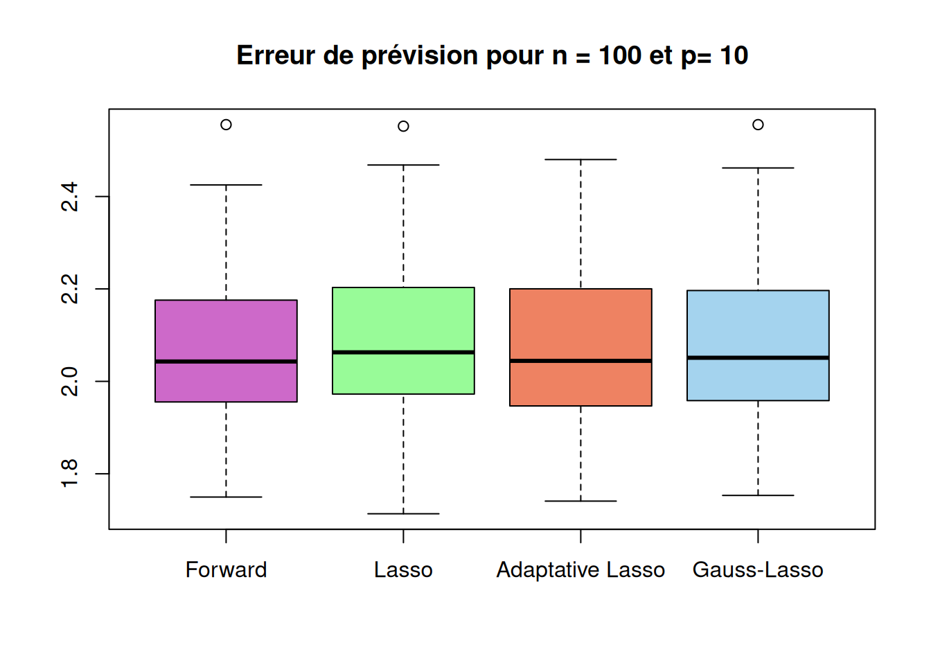

Show the code

res_cas2 = data.frame(
  Method = c("Forward", "Lasso", "Adaptative Lasso", "Gauss-Lasso"), 
  Quality_of_selection = c(r_cas2$selec_method1,r_cas2$selec_method2,r_cas2$selec_method3,NA),
  Mean_nb_selected_var = c(mean(r_cas2$taille_method1),mean(r_cas2$taille_method2),mean(r_cas2$taille_method3),NA),
  Prevision_error = c(mean(r_cas2$prev_method1),mean(r_cas2$prev_method2),mean(r_cas2$prev_method3),mean(r_cas2$prev_method4)),
  Running_time = c(r_cas2$temps1,r_cas2$temps2,r_cas2$temps3,r_cas2$temps4)
)
t(res_cas2)

                     [,1]       [,2]       [,3]               [,4]         
Method               "Forward"  "Lasso"    "Adaptative Lasso" "Gauss-Lasso"
Quality_of_selection "0.01"     "0.01"     "0.10"             NA           
Mean_nb_selected_var " 8.11"    "14.59"    " 7.61"            NA           
Prevision_error      "5.682778" "4.824673" "4.588443"         "5.223387"   
Running_time         "0.13837"  "0.06476"  "0.09358"          "0.09517"

Show the code

boxplot(sqrt(r_cas2$prev_method1),sqrt(r_cas2$prev_method2),sqrt(r_cas2$prev_method3),sqrt(r_cas2$prev_method4),
        names=c("Forward","Lasso","Adaptative Lasso","Gauss-Lasso"),
        main=paste("Erreur de prévision pour n =", n,"et p=", p_list[2]),
        col = c("orchid3", "palegreen", "salmon2", "lightskyblue2"))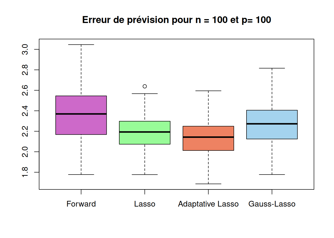

Show the code

res_cas3 = data.frame(
  Method = c("Forward", "Lasso", "Adaptative Lasso", "Gauss-Lasso"), 
  Quality_of_selection = c(r_cas3$selec_method1,r_cas3$selec_method2,r_cas3$selec_method3,NA),
  Mean_nb_selected_var = c(mean(r_cas3$taille_method1),mean(r_cas3$taille_method2),mean(r_cas3$taille_method3),NA),
  Prevision_error = c(mean(r_cas3$prev_method1),mean(r_cas3$prev_method2),mean(r_cas3$prev_method3),mean(r_cas3$prev_method4)),
  Running_time = c(r_cas3$temps1,r_cas3$temps2,r_cas3$temps3,r_cas3$temps4)
)
t(res_cas3)

                     [,1]        [,2]        [,3]               [,4]         
Method               "Forward"   "Lasso"     "Adaptative Lasso" "Gauss-Lasso"
Quality_of_selection "0.00"      "0.01"      "0.16"             NA           
Mean_nb_selected_var "48.66"     "17.34"     " 7.73"            NA           
Prevision_error      "11.428807" " 5.016189" " 4.523595"        " 5.243494"  
Running_time         "2.67996"   "0.06936"   "0.10052"          "0.10242"

Show the code

boxplot(sqrt(r_cas3$prev_method1),sqrt(r_cas3$prev_method2),sqrt(r_cas3$prev_method3),sqrt(r_cas3$prev_method4),
        names=c("Forward","Lasso","Adaptative Lasso","Gauss-Lasso"),
        main=paste("Erreur de prévision pour n =", n,"et p=", p_list[3]),
        col = c("orchid3", "palegreen", "salmon2", "lightskyblue2"))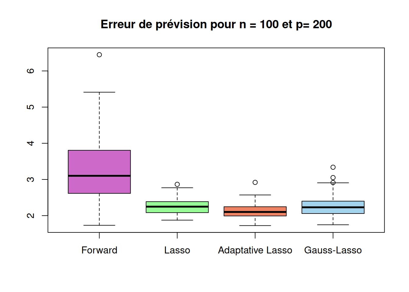

Show the code

res_cas4 = data.frame(
  Method = c("Forward", "Lasso", "Adaptative Lasso", "Gauss-Lasso"), 
  Quality_of_selection = c(r_cas4$selec_method1,r_cas4$selec_method2,r_cas4$selec_method3,NA),
  Mean_nb_selected_var = c(mean(r_cas4$taille_method1),mean(r_cas4$taille_method2),mean(r_cas4$taille_method3),NA),
  Prevision_error = c(mean(r_cas4$prev_method1),mean(r_cas4$prev_method2),mean(r_cas4$prev_method3),mean(r_cas4$prev_method4)),
  Running_time = c(r_cas4$temps1,r_cas4$temps2,r_cas4$temps3,r_cas4$temps4)
)
t(res_cas4)

                     [,1]        [,2]        [,3]               [,4]         
Method               "Forward"   "Lasso"     "Adaptative Lasso" "Gauss-Lasso"
Quality_of_selection " 0"        " 0"        " 0"               NA           
Mean_nb_selected_var "99"        "11"        " 6"               NA           
Prevision_error      "11.946047" " 5.699005" " 4.413508"        " 5.439750"  
Running_time         "61.347"    " 0.088"    " 0.129"           " 0.133"

Show the code

res_cas4bis = data.frame(
  Method = c("Forward", "Lasso", "Adaptative Lasso", "Gauss-Lasso"), 
  Quality_of_selection = c(r_cas4bis$selec_method1,r_cas4bis$selec_method2,r_cas4bis$selec_method3,NA),
  Mean_nb_selected_var = c(mean(r_cas4bis$taille_method1),mean(r_cas4bis$taille_method2),mean(r_cas4bis$taille_method3),NA),
  Prevision_error = c(mean(r_cas4bis$prev_method1),mean(r_cas4bis$prev_method2),mean(r_cas4bis$prev_method3),mean(r_cas4bis$prev_method4)),
  Running_time = c(r_cas4bis$temps1,r_cas4bis$temps2,r_cas4bis$temps3,r_cas4bis$temps4)
)

Warning in mean.default(r_cas4bis$taille_method1): l'argument n'est ni
numérique, ni logique : renvoi de NA

Warning in mean.default(r_cas4bis$prev_method1): l'argument n'est ni numérique,
ni logique : renvoi de NA

Show the code

t(res_cas4bis)

                     [,1]      [,2]       [,3]               [,4]         
Method               "Forward" "Lasso"    "Adaptative Lasso" "Gauss-Lasso"
Quality_of_selection NA        "0.00"     "0.03"             NA           
Mean_nb_selected_var NA        "30.92"    "11.07"            NA           
Prevision_error      NA        "5.260876" "4.776523"         "5.836417"   
Running_time         NA        "0.08522"  "0.13196"          "0.13632"

Show the code

boxplot(sqrt(r_cas4$prev_method1),sqrt(r_cas4$prev_method2),sqrt(r_cas4$prev_method3),sqrt(r_cas4$prev_method4),
        names=c("Forward","Lasso","Adaptative Lasso","Gauss-Lasso"),
        main=paste("Erreur de prévision pour n =", n,"et p=", p_list[3]),
        col = c("orchid3", "palegreen", "salmon2", "lightskyblue2"))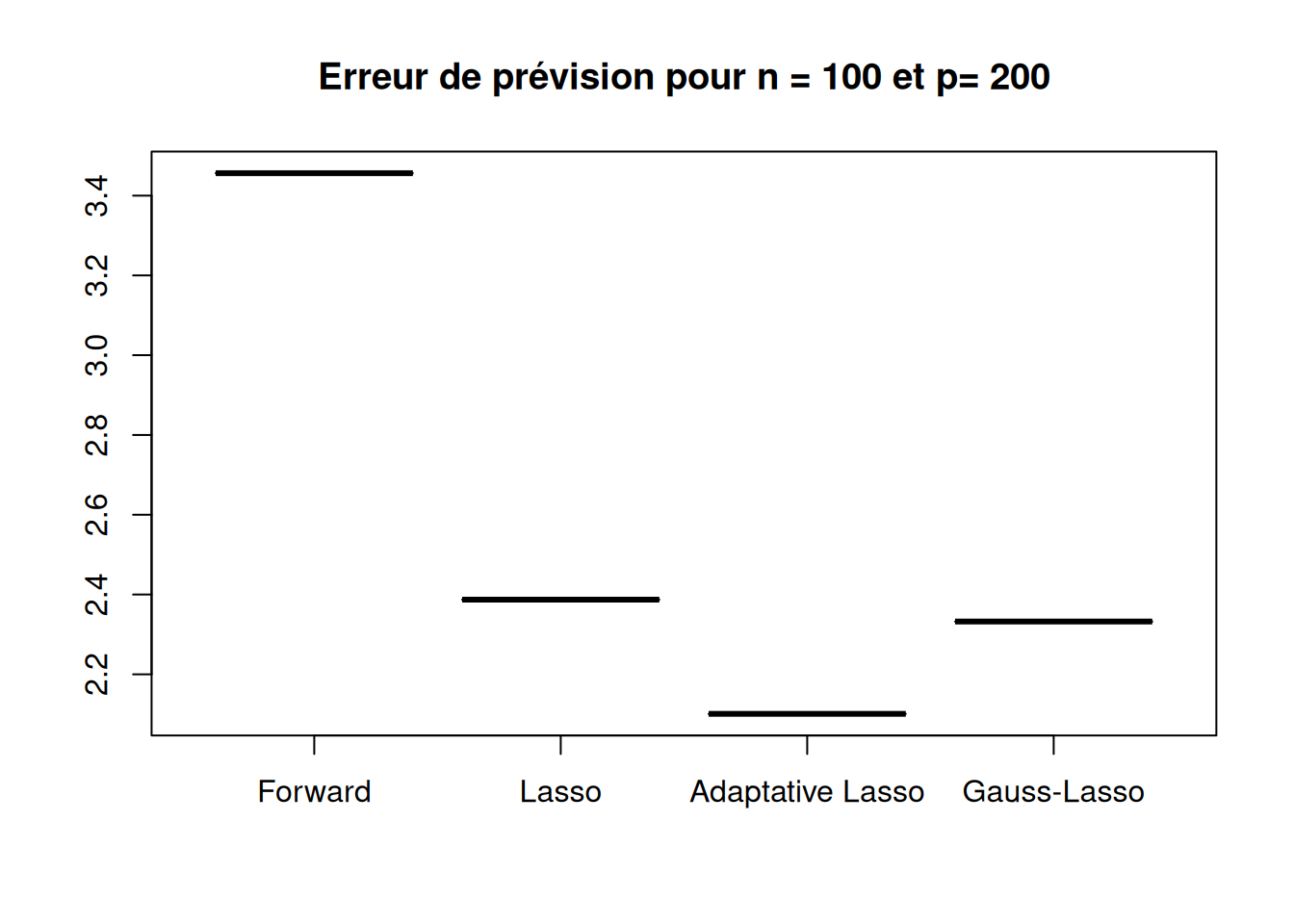

Show the code

boxplot(sqrt(r_cas4$prev_method1),sqrt(r_cas4bis$prev_method2),sqrt(r_cas4bis$prev_method3),sqrt(r_cas4bis$prev_method4),
        names=c("Forward","Lasso","Adaptative Lasso","Gauss-Lasso"),
        main=paste("Erreur de prévision pour n =", n,"et p=", p_list[4]),
        col = c("orchid3", "palegreen", "salmon2", "lightskyblue2"))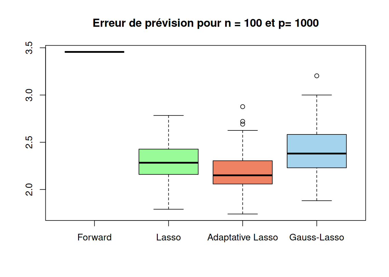

Question 7

Conclure sur les mérites respectifs de chaque méthode dans le contexte de l’étude.

Question 8

Quelles autres types de simulations pourrait-on envisager pour confirmer ou affiner ces conclusions ?